Support Vector Machines

Two-category data that can be cleanly divided by a single line with no misclassifications is called linearly separable. The data below are linearly separable. Given the lines shown in the image, the middle line best separates the data.

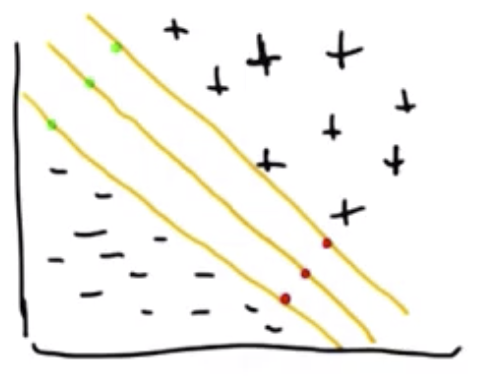
The other two lines are more likely to be overfit to the data. They may “believe the data too much.” A specific way of articulating this is to say the middle line is consistent with the data, while committing least to it.

Hyperplane Derivation

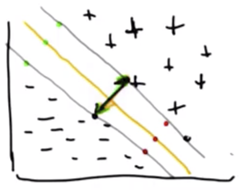
In the example shown below, one can imagine the two grey lines as boundary lines beyond which misclassifications would occur. The line in the middle is the best separator because it leaves the maximum space between these hypothetical boundary lines.

The general equation of a line is $y = mx + b$.

But, we are interested in a formulation that would allow for a more general case that would work with hyperplanes. In particular, this generalized equation follows:

$$y = w^Tx + b$$

where:

• $y$ are the classification labels that indicates which class the data is in, specifically, $y \in \lbrace-1,1\rbrace$
  
• $w^T$ are parameters of the plane, and
  
• $b$ are parameters of the plane that specifically translate the plane away from the origin.

The actual equation of the separating hyperplane would be given by the following, because this is where the output would be zero.

$$w^Tx + b = 0$$

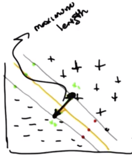
The top and bottom grey lines in the following figure are given by $w^Tx_1+b=1$ and $w^Tx_2+b=-1$, respectively.

Margin Derivation

The objective, for reasons previously outlined, is to have a support vector machine with the maximum possible distance between the grey hyperplanes. To find an equation for this distance, we subtract the equations listed above from one another, resulting in:

$$w^T(x_1-x_2)=2$$

Next, divide by the length of the vector $w$. The resulting formula is the distance between the hyperplanes, called the margin, denoted $m$:

$$m = \frac{w^T}{||w||}(x_1-x_2)=\frac{2}{||w||}$$

Again, the whole notion of finding the optimum decision boundary is the same as finding a line that maximizes the margin, while classifying everything correctly.

Maximizing the Margin

“Classifying everything correctly” is expressed mathematically as:

$$y_i(w^tx_i + b) \geq 1 \ \ \ \forall_i$$

Maximizing $\frac{2}{||w||}$ is the same as minimizing $\frac{1}{2}||w||^2$, which is easier to solve due to its being a “quadratic programming problem,” which is solvable in a relatively straightforward way.

Further, minimizing $\frac{1}{2}||w||^2$ is the same as maximizing the following function, for reasons not discussed in the lecture. Recall that $x$ are the datapoints, $y$ are the data labels.

$$W(\alpha)=\sum_i \alpha_i - \frac{1}{2} \sum_i \alpha_i \alpha_j y_i y_j x_i^T x_j$$

such that $\alpha_i \geq \phi$ and $\sum_i \alpha_i y_i = \phi$.

The solution to the foregoing equation has the following properties.

• Once $\alpha$ has been solved for, $w$ can likewise be solved: $w = \sum_i \alpha_i y_i x_i$. Once $w$ has been solved, it is easy to recover $b$.
• $\alpha_i$ are mostly 0. A logical result is that only a few of the vectors, $x_i$, in the previous bullet actually matter, and the “machine” only requires a few “support vectors.” The support vectors are the vectors for which $\alpha_i \neq 0$.
  • The support vectors are the vectors near the decision boundary, which actually constrain the line. This makes support vector machines conceptually similar to k-nearest neighbors, except that some work is done up front to compute which points matter.
• The $x_i^T x_j$ part of the $W(\alpha)$ function is a dot product of those two vectors, which is essentially a measure of their similarity.

Linearly Married

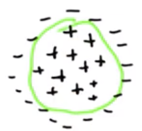
As example of a set of linearly married points is shown below. The idea is that there is no linear separator that can drawn to correctly classify the points.

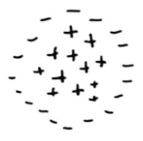
In order to use SVMs with data like that shown above, it must be transformed. The original 2-dimensional points, $q = \langle q_1, q_2 \rangle$, are transformed into a 3-dimensional space, as outlined below.

$$\Phi(q) = \langle q_1^2, q_2^2, \sqrt{2}q_1q_2 \rangle$$

Example

As an example, consider the following two data points $x = \langle x_1, x_2 \rangle$, $y = \langle y_1, y_2 \rangle$. How would we compute the dot product of those two points, but passed through the function $\Phi(q)$?

The dot product of two points is given by $x^Ty$, and the but first they must be passed through the transformation.

$$\Phi(x)^T \Phi(y)$$

$$ = \langle x_1^2, x_2^2, \sqrt{2} x_1 x_2 \rangle ^T \langle y_1^2, y_2^2, \sqrt{2} y_1 y_2 \rangle$$

$$ = x_1^2 y_1^2 + 2 x_1 x_2 y_1 y_2 + x_2^2 y_2^2 $$

$$ = (x_1 y_1 + x_2 y_2)^2 $$

$$ = (x^T y)^2 $$

Which, itself, is the dot product of $x$ and $y$. $x^T y$ is a particular form for the equation of a circle.

This means we have transformed from thinking about the linear relationship between the datapoints to thinking about something that looks a lot more like a circle. The notion of similarity, as captured by $x^T y$, is, again, now more like a circle, $(x^T y)^2$.

In this specific example, all the minuses move “up,” out of the screen, a lot. The pluses, being closer to the origin, move up less. As a result, the data can be cleanly separated by a hyperplane.

Additionally, in the case of transforming $x^Ty$ into $(x^Ty)^2$, rather than actually projecting each of the points into the third dimension, we simply replace the former with the latter in this formulation of the quadratic program: $W(\alpha)=\sum_i \alpha_i - \frac{1}{2} \sum_i \alpha_i \alpha_j y_i y_j x_i^T x_j$.

Then, it is as if we had projected all of the data into this third dimension, but in reality, we never used the function $\Phi$.

This (kind of) transformation into a higher dimensional space in order to separate the data is called a “Kernel Trick.”

Kernel Trick

The actual “Kernel” is the function $K(x_i,x_j)$ in the quadratic program:

$$W(\alpha)=\sum_i \alpha_i - \frac{1}{2} \sum_i \alpha_i \alpha_j y_i y_j K(x_i,x_j)$$

The Kernel takes the parameters $x_i$ and $x_j$ and returns some number.

• The Kernel function is our representation of similarity between those two points.
• It is also a mechanism by which we inject domain knowledge into the support vector machine learning algorithm.

There are several types of kernels, including:

• Polynomial kernel: $K=(x^Ty+c)^P$
• Radial basis kernel: $e^{\frac{{||x-y||}^2}{2 \sigma^2}}$
• Sigmoid kernel: $tanh(\alpha x^Ty+\theta)$

Since the Kernels are just arbitrary functions that return a number, $x$ and $y$ do not need to be points in a continuous number space. They could be discrete values, strings, images, etc.

Mercer Condition

The Mercer Condition is a technical condition, but in essence it means that the Kernel function must act like a well-behaved distance function. This is the only real criterion a Kernel function, generally, must meet.