Regression & Classification
Regression is an example of supervised learning. Recall that supervised learning which is a paradigm in which examples of inputs and outputs are generalized to predict outputs for new inputs.
Regression is a special subtopic because it involves mapping continuous inputs (as opposed to discrete inputs) to outputs.
Regression to the Mean
When tall people have children, their children, on average, tend to be have heights somewhere in between the height of their parents and the average height of the population. This is an example of regressing to the mean, and is shown diagrammatically in the image below. The slop of the line is $\frac{2}{3}$, which indicates that tall people tend to have children that are slightly shorter than they are, but still taller than average.
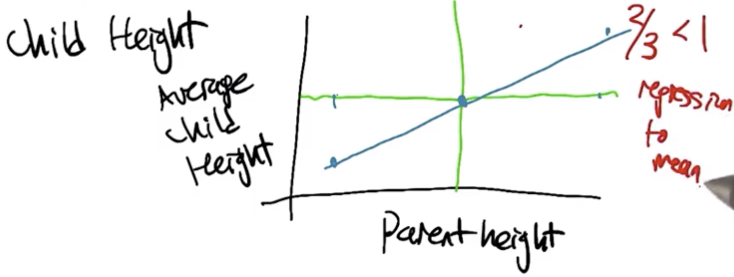
Regression to the mean has now come to refer more generically to the process of approximating a functional form using a set of datapoints. Strictly speaking, nothing is “regressing” with this usage of the term, but the term has stuck.
Best Fit Lines
Finding the Best Fit Line for a set of datapoints is accomplished using Calculus. Specifically, it is accomplished by minimizing the sum of the squared errors.
For a constant function, like the one shown in red below, $$f(x)=c$$ this is found by minimizing the sum of squared errors which are shown in green, $$E(c)=\sum_{i=1}^{n} (y_i-c)^2$$
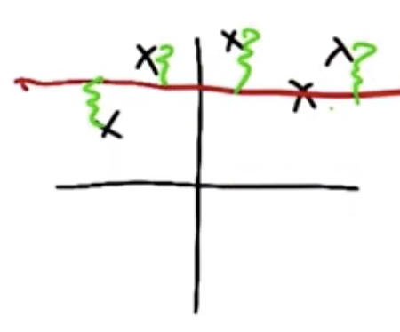
Another generalized term for the error function is the “loss” function. To solve for the value of $c$ that minimizes the error, we take the derivative of the loss function $E(c)$, set equal to zero, and solve for $c$.
$$\frac{dE(c)}{dc} = \sum_{i=1}^{n} 2(y_i-c)(-1) = 0$$
In this case, the constant $c$ that minimizes error is the mean:
$$c=mean(y)=\sum_{i=1}^{n} \frac{y_i}{n}$$
Order of Polynomial
- k = 0: constant,
- k = 1: line,
- k = 2: parabola
$$f(x) = c_0 + c_1 x + c_2 x^2 + … + c_k x^k$$
The three orders of polynomials listed above are shown graphically, below, for the dataset shown.
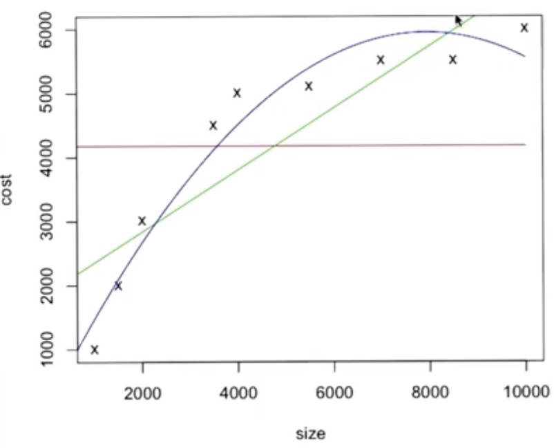
The order of the polynomial used to fit the line cannot exceed the number of datapoints - 1, in the case of the data shown above this is 8.
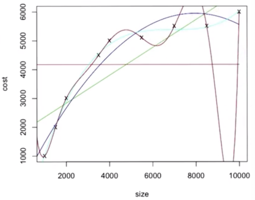
The best line to use is the light blue cubic. Note that the red octic overfits the data.
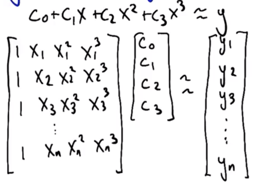
The matrix multiplication shown above is represented more simply by:
$$X w \approx Y$$
where $w$ is the coefficients, which are solved for as follows:
$$X^T X w \approx X^T Y$$ $$(X^T X)^{-1} X^T w \approx (X^T X)^{-1} X^T Y$$ $$w = (X^T X)^{-1} X^T Y$$
Errors
Training data always has errors. It includes the underlying function, $f$, but some error component, $\epsilon$, as well. So, the training data is $f + \epsilon$. What are the various soruces for this error?
- Sensor error - inherent in machinery
- Malicious error - being given bad data
- Transcription error - humans transposing values or writing data incorrectly
- Unmodeled Influences - housing data shown above only included the size of the house and the price. Many other items would also influence the price of the house:
- Location, location, location
- Quality of house
- Builder of the house
- Interest rates
Cross Validation
A fundamental assumption of all machine learning activities is that the training set and test set are representative of the real world data on which the machine learning algorithm will operate. Statisticians use the abbreviation IID (Independent, and Identically-Distributed), which means the data that is being used comes from the same source.
A goal of machine learning is to use a model that is complex enough to fit the training set without causing problems on the test set. One way to ensure this is to use a cross validation test set, which is a part of the training set that is set apart for purposes of checking the model without officially testing using the test set.
Practically, this involves splitting the training set into several folds:
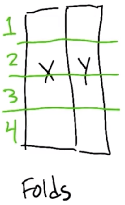
| Training Set | Cross-Validation Set |
|---|---|
| 1, 2, 3 | 4 |
| 2, 3, 4 | 1 |
| 3, 4, 1 | 2 |
| 4, 1, 2 | 3 |
The cross-validation approach involves:
- Training on each of the training subset, and
- Calculating the error on each cross-validation set.
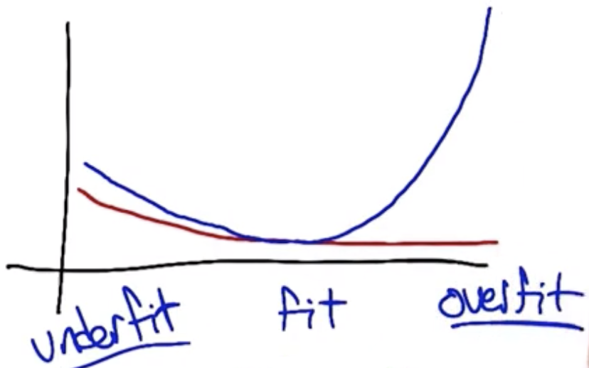
Once complete, the errors on the cross-validation set are averaged to determine overall error for the model used. The model class (for example, the polynomial order) that minimizes the error is the class that should be used. In the graphic below, the training error improves with increasing in the polynomial degree, but beyond degree 4 the cross-validation error begins increasing.
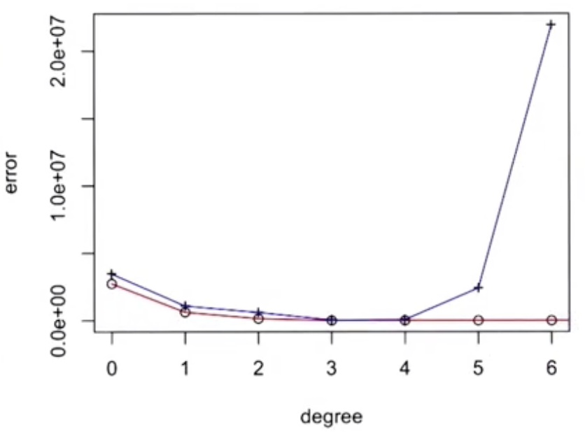
In the example shown above, the optimal model appears to be a polynomial of degree 3.
Other Input Spaces and Representations
- Continuous Scalar input: $x$ examples so far
- Continuous Vector input: $\vec{x}$ - also possible, could include more input features:
- Size,
- Distance from Zoo
Raises question of encoding discrete categorical inputs that will be considered in subsequent lectures:
- Considerations for Predicting Credit Score:
- Job?
- Age?
- Assets?
- Type of Job?
For Fall 2019, CS 7461 is instructed by Dr. Charles Isbell. The course content was originally created by Dr. Charles Isbell and Dr. Michael Littman.