Probability Density Functions
As there are many ways of describing data sets, there are analogous ways of describing histogram representations of data.
These representations are termed “discrete” probability distributions, as distinct from “continuous” probability distributions which are also known as “Probability Density Functions” and discussed later.
Histograms
A histogram is a way of visually representing sets of data. Specifically, it is a bar chart of frequency in which data appears within certain ranges (or “bins”).
In general, there are two types of histograms. The first is called a “Frequency histogram” and has counts of occurrences on the Y-axis. The second is called a “Probability histogram” and has probabilities on the Y-axis. Examples of both types, generated from the same set of 125 data points, are shown below.
The data are a series of 125 values, the first five of which are: $-0.023, -0.095, -0.204, \ 0.004, -0.063$.
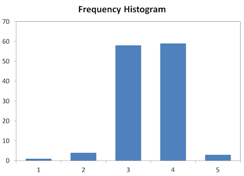
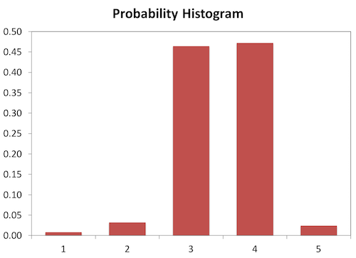
| Bin | Low | High | Count | “Probability,” p_i | Midpoint, x_i |
|---|---|---|---|---|---|
| 1 | -0.3 | -0.2 | 1 | 0.008 | -0.25 |
| 2 | -0.2 | -0.1 | 4 | 0.032 | -0.15 |
| 3 | -0.1 | 0 | 58 | 0.464 | -0.05 |
| 4 | 0 | 0.1 | 59 | 0.472 | 0.05 |
| 5 | 0.1 | 0.2 | 3 | 0.024 | 0.15 |
Histogram Descriptions
The example used for the following calculations is the “Probability Histogram” with red bars, above.
$p_i$ is the probability associated with each bin. $x_i$ is the midpoint of each bin. $\mu$ is the weighted average mean of the bins, calculated as follows.
Mean
$$\text{mean} = \mu = \sum_{i=1}^{bin\ count} (p_i)(x_i)$$
$$\mu_x = \frac{1}{n} \sum_{i=1}^n x_i = 44.67$$
In this case, it is calculated as follows.
$$\mu=(0.008)(-0.25)+…+(0.024)(0.15)=-0.0028$$
Variance
The variance of a bin is calculated as follows. This parameter is also known as the 2nd moment about the mean. The standard deviation of the histogram can be calculated as the squire root of the variance.
$$\text{variance}=\sum_{i=1}^{bin\ count}{p_i (x_i-\mu)^2}$$
For this histogram, the variance is 0.0041.
Skewness
Skewness is the 3rd moment about the mean.
$$skewness=\sum_{i=1}^{bin\ count} {p_i (x_i-\mu)^3}$$
For this histogram, the skewness is -0.00012.
Kurtosis
Kurtosis is the 4th moment about the mean.
$$\text{kurtosis}=\sum_{i=1}^{bin\ count}{p_i (x_i-\mu)^4}$$
Probability Density Functions
Continuous probability distributions have the property of always having area 1 under the curve. Expressed mathematically, this is written:
$$\int{f(x)}dx=1$$
The properties for continuous probability distributions are analogous to those discrete distributions:
$$\text{mean}=\int{f(x)xdx}$$
$$\text{variance}=\int{f(x)(x-\mu)^2dx}$$
$$\text{skewness}=\int{f(x)(x-\mu)^3dx}$$
Important and Common PDFs
Many phenomenon described by data closely approximate certain distributions. In many situations, there are certain distributions that should be chosen, if we are ignorant of the true distribution. These representations are most appropriate because they are the representations that have maximum entropy (or uncertainty).
Support Set: the set over which the distribution is defined.
Uniform Continuous Distribution
Support set: real number line from a to b
$$f(x)=\frac{1}{b-a}$$
$$\text{mean}=\frac{a+b}{2}$$
$$\text{variance}=\frac{(b-a)^2}{12}$$
$$\text{skewness}=0$$
$$\text{entropy}=log_2(b-a)$$
The uniform continuous distribution is the maximum entropy distribution for $a$ and $b$ finite and known.
Uniform Discrete Distribution
Support set: discrete numbers from a to b
$$f(x)=\text{discrete values a to b}$$
$$\text{mean}=\frac{a+b}{2}$$
$$\text{variance}=\frac{(b-a+1)^2-1}{12}$$
$$\text{skewness}=0$$
$$\text{entropy}=log\ n$$
This is the appropriate choice where something can take any value between a minimum and a maximum, but the values are discrete (IE, must be represented by a whole number).
Gaussian Continuous Probability Density Function
Support set: $(-\infty,\infty)$
$$f(x)=\frac{1}{\sqrt{2\pi\sigma^2}}\int{e^{\frac{-(x-\mu)^2}{2\sigma^2}}dx}$$
$$\text{mean}=\mu$$
$$\text{variance}=\sigma^2$$
$$\text{skewness}=0$$
$$\text{entropy}=2.05+log{\ \sigma}$$
When there is a distribution that can take any value from $(-\infty,\infty)$ and all that is known is the standard deviation, $\sigma$ or variance $\sigma^2$, this is the maximum entropy distribution. This means that if we have complete ignorance of a phenomenon, except for its variance, then we should use a Gaussian.
Histograms Spreadsheet.xlsx
Some other content is taken from my notes on other aspects of the Coursera course.