Linear Regression and Standardization
Linear regression is a more informative metric for evaluating associations between variables than most people typically realize. When it is used to forecast outcomes, it can be converted to a measure of information gain or converted into a point estimate and associated confidence interval. It can also be used to quantify the amount a linear model reduces uncertainty.
Linear regression is closely related to the Central Limit Theorem because both regression and the CLT use probability distributions known as “Gaussians.”
Standardization
Standardizing a set of values requires calculating the mean, $\mu_x$, and standard deviation of the population, $\sigma_x$. The appropriate excel formulae are STDEVP and AVERAGE. By convention, the raw data values are denoted $x_i$, and the standardized values are denoted $x_{zi}$.
$$\mu_x = \frac{1}{n}\sum_{i=1}^n x_i$$
$$\sigma_x = \sqrt{\frac{1}{n}\sum_{i=1}^n (x_i-\mu_x)^2}$$
$$x_{zi}=\frac{x_i-\mu_x}{\sigma_x}$$
In excel, standardization can be accomplished using the STANDARDIZE function, which takes as parameters the array of values to be standardized as well as the average and standard deviation thereof.
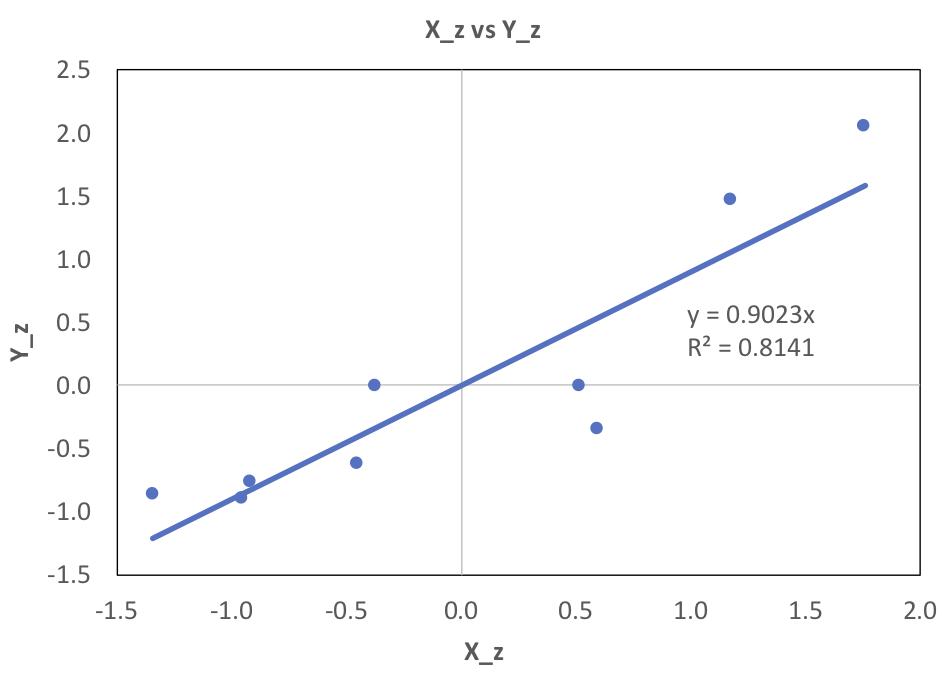
As an example, note that in the following standardization, both $X_z$ and $Y_z$ have the same standard deviation and mean, despite the X values having a much larger range of values. This is what is meant by standardization.
| X | Y | X_z | Y_z | |
|---|---|---|---|---|
| Values | 10 | 1.5 | -1.3 | -0.9 |
| 90 | 10.0 | 1.8 | 2.0 | |
| 75 | 8.3 | 1.2 | 1.5 | |
| 35 | 4.0 | -0.4 | 0.0 | |
| 20 | 1.4 | -1.0 | -0.9 | |
| 21 | 1.8 | -0.9 | -0.8 | |
| 33 | 2.2 | -0.5 | -0.6 | |
| 58 | 4.0 | 0.5 | 0.0 | |
| 60 | 3.0 | 0.6 | -0.4 | |
| μ | 44.7 | 4.02 | 0 | 0 |
| σ | 25.8 | 2.92 | 1 | 1 |
$$\mu_x=44.7,\ \mu_y=4.02,\ \mu_{xz}=0,\ \mu_{yz}=0$$
$$\sigma_x=25.8,\ \sigma_y=2.92,\ \sigma_{xz}=1,\ \sigma_{yz}=1$$

Next, I will consider how standardization affects certain relationships between sets of values, like covariance, correlation, slope and y-intercept of the best fit line.
Covariance
Covariance ($\text{Cov}$) is calculated as follows. The appropriate excel function is COVARIANCE.P.
$$\text{Cov}_{xy}=\frac{1}{n}\sum_{i=1}^n(x_i-\mu_{xi})(y_i-\mu_{yi})$$
The covariance of the raw data, above, is 67.89. The covariance of the standardized data is 0.902.
Best Fit Line
The best fit line for the relationship between two sets of data is commonly represented as follows.
$$\hat{y_i}=\beta x_i + \alpha$$
$\hat{y_i}$ represents the y-values that form the line of best fit. The slope of the best fit line is commonly represented by $\beta$. The appropriate excel function is SLOPE. The values are 0.102 and 0.902 for the raw and standardized data, respectively. Note that the covariance is the same as the $\beta$ for standardized data.
The y-intercept is commonly represented by $\alpha$. The appropriate excel function is INTERCEPT. The values are -0.535 and 0 for the raw and standardized data, respectively. Note that standardized data will always have a y-intercept of zero. This is because the point $(\mu_x,\mu_y)$ is always on the best fit line, and for standardized data that point is (0,0).
Correlation
Correlation is a function of the covariance and standard deviations of the data, calculated as follows. It is commonly represented as $R$, and sometimes known as the Pearson correlation coefficient or Pearson R test. The appropriate excel function is CORREL.
$$\text{R}=\frac{\text{Cov}_{xy}}{\sigma_{x}\sigma_{y}}$$
The correlation for two sets of data is the same whether they have been standardized or not. In the case of the data tabulated above, the correlation is 0.902.
Standardization Summary
The values discussed above are broken out, below.
| Raw Data | Standardized Data | |
|---|---|---|
| Covariance, Cov | 67.9 | 0.902 |
| Slope, Beta, β | 0.102 | 0.902 |
| Intercept, α | -0.535 | 0 |
| Correlation, R | 0.902 | 0.902 |
Note that the only values that are unchanged following standardization is the correlation. Note also that for standardized data the covariance and slope are equal to the correlation. That is, for standardized data,
$$\text{Cov}=\beta=R$$
Linear Regression
The goal of linear regression is to minimize the sum of squared errors (or “residuals”), where the sum of squared errors is given by
$$\sum{(y_i-\hat{y_i})^2}\ \ \ or\ \ \ \sum{e^2}$$
It can be shown that the standard deviation of residuals is the same as the root mean square of the residuals. Or:
$$\sigma_e=\sqrt{\frac{1}{n}\sum{e}}$$
Modeling Error using Linear Regression
It is possible to relate the variance of the error, $\sigma_e$, directly to the correlation and slope of the best fit line. Doing so requires making the assumption that the X and Y values are samples that are drawn from normally distributed data with $\mu = 0$ and $\sigma = 1$.
The actual y-values can be computed from the following.
$$Y\ values = (\beta)(X\ values) + error\ term$$
With the assumption of normally distributed data, this converts to the following.
$$\phi(0,\sigma_y^2)=\phi(0,\beta^2\sigma_x^2)+\phi(0,\sigma_e^2)$$
If the data is standardized, then $\sigma_y^2=\sigma_x^2=1$ and the previous formula reduces to the following.
$$1=\beta^2+\sigma_e^2$$
For standardized data, $\beta = R$, so
$$1=R^2+\sigma_e^2$$
This formula tells us there is a direct relationship between the standard deviation of the errors and the correlation. This is important because it enables us to make forecasts in the form of a probability distribution, not just a single point.
So, a forecast might take the form of a point value $\hat{y_i}=\beta x_i$ with standard deviation $\sigma_e$.
Example 1
Consider a situation where a 90% confidence interval is desired, and the data is correlated with $R=0.7$.
A 90% confidence interval translates to z-scores of 1.64 and -1.64. We calculate $\sigma_e=0.71$, then the 90% confidence interval is given by
$$\hat{y_i}=\beta x_i\pm(1.64)(.71)$$
Example 2
A data analysis model has a standard deviation of model error of $2500 at a correlation of R = 0.30. The model needs to be improved to the point that the standard deviation of model error is $1500.
Using the formula $1=R^2+\sigma_e^2$, $\sigma_e$ is solved to be 0.954. Then the required $\sigma_e$ is calculated as follows:
$$\sigma_{e,required}=\frac{1500}{2500}\sigma_{e,actual}=.572$$
$$R_{e,required} = \sqrt{1-\sigma_{e,required}^2}=.82$$
Connection to Mutual Information
It is possible to demonstrate that, in a parametric model that has Gaussian distributions, the mutual information is given by
$$I(X;Y)=log(\frac{1}{\sqrt{1-R^2}})$$
Thus, for a parameterized Gaussian model with continuous distributions, if the correlation between X and Y,
$R$, increases, the percentage information gain also increases, becoming infinite at R=1.
Standardization-Spreadsheet.xlsx
Correlation-and-Model-Error.xlsx
Correlation-and-P.I.G.xlsx
Some other content is taken from my notes on other aspects of the Coursera course.