Gaussian Distribution
Linear regression is a more informative metric for evaluating associations between variables than most people typically realize. When it is used to forecast outcomes, it can be converted to a measure of information gain or converted into a point estimate and associated confidence interval. It can also be used to quantify the amount a linear model reduces uncertainty.
Linear regression is closely related to the Central Limit Theorem because both regression and the CLT use probability distributions known as “Gaussians.”
Gaussian Distributions
Diligent data analysts will always include a model of the remaining uncertainty (or noise) associated with their conclusions and recommendations. Any given data analysis will include “signal” and “noise.” Noise is defined as that part of the future that cannot be explained by the present data. Examples include the uncertainty associated with forecasts from a linear regression model, or the uncertainty about a financial instrument’s rate of return. Noise cannot be eliminated completely.
Gaussian Probability Density (or “Normal”) functions are by far the most common model for uncertainty (or noise) used in data analysis. It is a type of continuous distribution that has many special properties.
Standardization
There are 3 steps to standardizing data:
- Calculate mean, variance, and, from it, standard deviation.
X Values = 10, 90, 75, 35, 20, 21, 33, 58, 60
Mean ( $\mu_x$ ):
$$\mu_x = \frac{1}{n} \sum_{i=1}^n x_i = 44.67$$
Population Variance:
$$\frac{1}{n} \sum_{i=1}^n {x_i - \mu_x}^2$$
Population Standard Deviation ($\sigma_x$, stdevp in Excel):
$$\sigma_x = \sqrt(\frac{1}{n}\sum_{i=1}^n (x_i - \mu_x)^2) = 25.79$$
- Subtract the mean from each value.
- Divide the resulting value by the standard deviation.
| X Values | 10 | 90 | 75 | 35 | 20 | 21 | 33 | 58 | 60 |
|---|---|---|---|---|---|---|---|---|---|
| Step 2 | -34.7 | 45.3 | 30.3 | -9.7 | -24.7 | -23.7 | -11.7 | 13.3 | 15.3 |
| Step 3 | -1.34 | 1.76 | 1.18 | -0.37 | -0.96 | -0.92 | -0.45 | 0.52 | 0.59 |
The resulting standardized values are denoted $x_{zi}$.
$$x_{zi}=\frac{x_i-\mu_x}{\sigma_x}$$
Note that this standardization process will always produce values with a mean of 0 and standard deviation of 1 ($\mu_{xz} = 0$ and $\sigma_{xz} = 1$).
Properties of the Standard Normal Distribution
- Standard Area = 1
- Mean = 0
- $\sigma = \sigma^2 = 1$
- Height of the curve is .399 or $\frac{1}{\sqrt{2\pi}}$
- Generated by the function $f(x)=\frac{1}{\sqrt{2*\pi}}e^-\frac{x^2}{2}$
- Area under curve is known as the cumulative probability distribution function, given by
$$\frac{1}{\sqrt(2\pi)} \int_{-\infty}^\infty{e^{-x^2 / 2}}dx$$
- To find the area to the left of a particular z-score, replace the upper limit of the integral, as follows:
$$\frac{1}{\sqrt{2\pi}}\int_{-\infty}^z{e^{-x^2 / 2}}dx$$
- In the figure below, the red distribution is a standard normal curve. We say $\phi(0,1)$. The green curve would be $\phi(-2,0.5)$. Note that all these curves have area = 1. Larger variance curves will be lower and flatter; small variance curves will be taller.
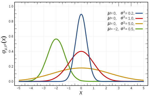
-
Most of the probability is in the middle of the distribution:
- At z=1, 84.1% of the probability is to the left.
- At z=2, 97.7%.
- At z=3, 99.8%.
- At z=4, 99.9968%.
-
In Excel,
NORMSDISTandNORMSINVfunctions calculate probabilities from z-scores and z-scores from probabilities, respectively. Probabilities are values in between 0 and 1, inclusive.
Example 1
As a practical example, assume that the standard deviation of a certain manufacturing process is known, and that the mean of the process needs to be set such that only one part in 10,000 falls below a certain minimum tolerance.
The mean should be placed =NORMSINV(1-(1/10000)) or 3.719 standard deviations above the minimum tolerance.
Example 2
As a further example, consider that a population of people have an average heart rate of 110 beats per minute with standard deviation of 15. They are given a medication. Following medication, a 45-person sample are measured to have an average heart rate of 102.
The sample standard deviation is calculated as $\frac{15}{\sqrt{45}}$ or 2.24. The z-score is calculated as $\frac{110-102}{2.24}$ or -3.58. The probability of that decrease in heart rate occurring by chance is 0.017%.
Central Limit Theorem
The Central Limit Theorem is an important reason for the Gaussian distribution’s prevalence in nature and in data. The Central Limit Theorem states that given any probability distribution with mean, $\mu$, and standard deviation, $\sigma$, taking samples (size, $n$, $\ge$ 30) from the distribution will have a few results:
- the mean of the sample means will approach the mean of the original distribution,
$$\mu_{\bar{x}}=\mu$$
- the standard deviation of sample means will approach the standard deviation of the original distribution divided by the square root of the size of the samples,
$$\sigma_{\bar{x}}=\frac{\sigma}{\sqrt{n}}$$
- and the histogram of sample means will form an approximate Gaussian distribution, independent of the shape of the original distribution.
In particular one formula that seems to occur frequently in Central Limit problems is the variance of a continuous uniform distribution from $x_{min}$ to $x_{max}$. The variance is given by
$$\frac{(x_{max}-x_{min})^2}{12}$$
Algebra Using Gaussians
Summation of Independent Distributions
Given the following two independent (no dependency, covariance, correlation) Gaussian distributions (note $\sigma^2$, variance, is the square of standard deviation, $\sigma$):
$$\phi_1(\mu_1,\sigma_1^2), \phi_2(\mu_2,\sigma_2^2)$$
Summing them will result in a distribution described as follows:
$$\mu_{1+2}=\mu_1+\mu_2$$
$$\sigma_{1+2}^2=\sigma_1^2+\sigma_2^2$$
Multiplying an Independent Distribution by a Constant ($\beta$)
Given a Gaussian distribution:
$$\phi_1(\mu_1,\sigma_1^2)$$
Multiplying a given term, $z$, by $\beta$ produces the following:
$$\phi_\beta=(\beta\mu_1,\beta^2\sigma_1^2)$$
Dependent Distributions
When covariance $\ne$ 0, then the distributions are dependent. Note, $w_1+w_2=1$. Then, combining the distributions results in the following standard variance.
$$\sigma_{1+2}^2=w_1^2\sigma_1^2+w_2^2\sigma_2^2+2w_1w_2\text{Cov}_{12}$$
Markowitz Portfolio Optimization Example
Markowitz Portfolio Optimization is an excellent example of the application of algebra using Gaussian distributions. The goal of Markowitz Portfolio Optimization is to create a combined portfolio of at least two investments that is optimal in a very specific way. Essentially, the optimization results in the largest possible returns-to-risk ratio.
For this example, the investments are stocks with expected returns, $ER_1$ and $ER_2$. The relative weighting of these investments are $w_1$ and $w_2$, where $w_1+w_2=1$.
Then, the return of the overall portfolio, plotted on the Y-Axis of the graph below, is given by:
$$ER_p=(w_1)(ER_1)+(w_2)(ER_2)$$
We are given that the covariance, $\text{Cov}$, is a function of the correlation, $R$, as expressed below. The correlation between two securities is more commonly available than the covariance.
$$\text{Cov}_{12}=R_{12} \sigma_1 \sigma_2$$
then, the volatility of returns for this portfolio, plotted on the X-Axis, is given by the weighted sum of the volatilities, combined as follows:
$$\sigma_p^2=w_1^2\sigma_1^2+w_2^2\sigma_2^2+2w_1w_2R_{12}\sigma_1\sigma_2$$
The data for this example are as follows:
| σ | ER | |
|---|---|---|
| Risk-Free Rate, rf | 0 | 0.01 |
| Stock 1 | 0.095 | 0.12 |
| Stock 2 | 0.083 | 0.10 |
Various weighted combinations of the two securities are plotted in yellow, below. The goal of Markowitz Portfolio Optimization is to maximize the Sharpe Ratio. This ratio is represented graphically as the slope of the dashed red line.
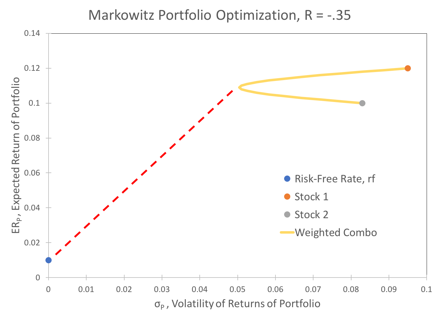
The Sharpe Ratio is written formulaically as
$$\text{Sharpe}=\frac{ER_p - r_f}{\sigma_p}$$
Performing the substitution:
$$\text{Sharpe}=\frac{(w_1)(ER_1)+(w_2)(ER_2)-r_f}{\sqrt{w_1^2\sigma_1^2+w_2^2\sigma_2^2+2w_1w_2R_{12}\sigma_1\sigma_2}}$$
With the information given in the problem, the Sharpe ratio becomes a function of two variables, $w_1$ and $w_2$, which are constrained by the relation $w_1 + w_2 = 1$. The “Solver” Excel plug-in can then be used to maximize the Sharpe ratio.
Taking this analysis a step further, $R_{12}$ can also be treated as a parameter of the Sharpe ratio. I consider five possible values for $R_{12}$, tabulated below. The results are a family of curves and Sharpe ratio lines, shown below. Using Solver, I optimize the weights, $w_1$ and $w_2$, for each of these R values, maximizing the Sharpe Ratio, and tabulate the results below the chart.
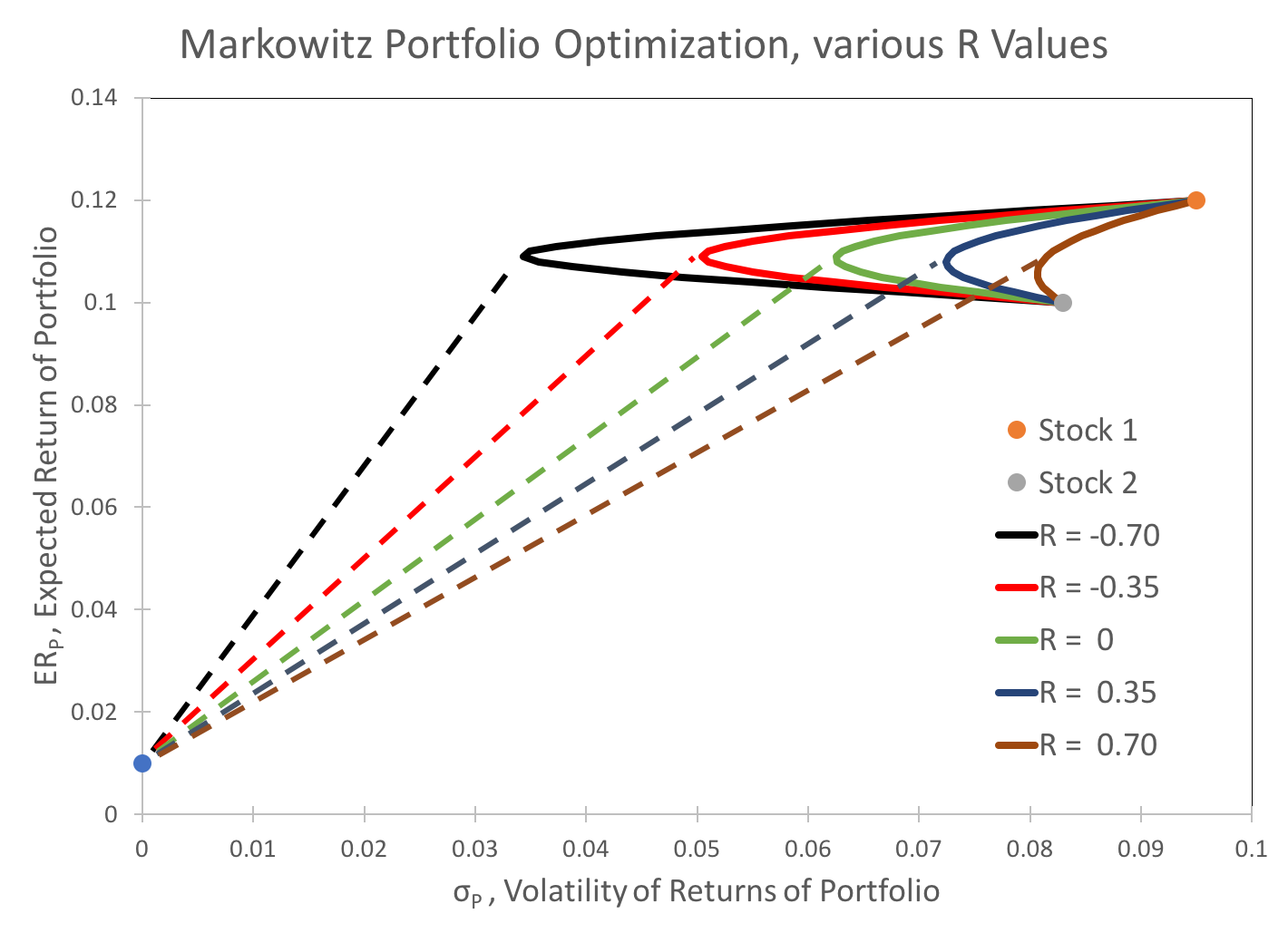
| R | Sharpe Ratio | w_1 | w_2 | ER_p | σ_p |
|---|---|---|---|---|---|
| -0.70 | 2.89 | 47% | 53% | 0.109 | 0.034 |
| -0.35 | 1.97 | 47% | 53% | 0.109 | 0.051 |
| 0.00 | 1.59 | 48% | 52% | 0.110 | 0.063 |
| 0.35 | 1.37 | 50% | 50% | 0.110 | 0.073 |
| 0.70 | 1.22 | 56% | 44% | 0.111 | 0.083 |
Note that, as expected, the volatility of returns is highly dependent on the amount of covariance. Interestingly, the optimal weighting for the securities is relatively stable, even given very wide swings in covariance. As a result, the expected returns are likewise relatively stable.
This analysis explains investors' constant search for diversification via alternative assets that are not highly correlated to major investment vehicles like the stock market.
Standardization-Spreadsheet.xlsx
Excel-NormS-Functions-Spreadsheet.xlsx
Typical-Problem-NormSDist-.xlsx
CLT-and-Excel-Rand.xlsx
Algebra-with-Gaussians.xlsx
Markowitz-Portfolio-Optimization.xlsx
Some other content is taken from my notes on other aspects of the aforementioned Coursera course.