Supervised Learning on Census Dataset
In this project, I employ several supervised learning algorithms to model individuals' income using data collected from the 1994 US Census. The goal of the project is to construct a model that accurately predicts whether an individual makes more than $50,000.
The result of the project is a model that is 87.1% accurate (75.4% F-score) at predicting whether an individual makes more than $50,000 based on 13 datapoints. Training the identical model on the most important 5 datapoints results in a model that is 85.9% accurate (72.8% F-score).
This is page 2 of 3 for the project, where I
Benchmark Several Default Machine Learning Models
The specific tasks break down as follows:
- Consider the performance of a Naive Predictor.
- Qualitatively analyze the suitability of each model to the dataset being explored.
- Create a Training and Predicting pipeline to facilitate quick training of several models using various sizes of training data.
- Select Top Model and discuss results.
%matplotlib inline

import pandas as pd
import matplotlib.pyplot as pl
import numpy as np

import matplotlib.patches as mpatches
y_train = pd.read_csv('processed/y_train.csv',
                      index_col=0)
y_test = pd.read_csv('processed/y_test.csv',
                     index_col=0)
y = y_train.append(y_test)
X_train = pd.read_csv('processed/X_train.csv',
                      index_col=0)
X_test = pd.read_csv('processed/X_test.csv',
                     index_col=0)
X = X_train.append(X_test)
Consider the Performance of a Naive Predictor
Remember the following definitions from a confusion matrix:
- True Positive: Both predicted and actually positive.
- True Negative: Both predicted and actually negative.
- False Negatives: Predicted negative, but actually positive.
- False Positive: Predicted positive, but actually negative.
$$Accuracy = \frac{TP+TN}{TP+TN+FP+FN}$$
$$Precision = \frac{TP}{TP+FP}$$
$$Recall = \frac{TP}{TP+FN}$$
$$F_{\beta}=(1+\beta^2) \cdot \frac{precision \cdot recall}{(\beta^2 \cdot precision) + recall}$$
- Precision focuses on the predicted positive values in the dataset.
- Recall focuses on the actually positive values in the dataset.
total = y['income'].count()
total_actual_positives = y['income'].sum()

print('      Total Datapoints: {}'.format(total))
print('Total Actual Positives: {}'.format(total_actual_positives))
print(' Actual Positive Ratio:    {:1.1%}'.format(total_actual_positives/total))
      Total Datapoints: 45222
Total Actual Positives: 11208
 Actual Positive Ratio:    24.8%
A naive predictor, in this case, would the entire dataset is positive. Note that this would clearly result in an accuracy less than 50%, since the actual positives are less than half of the total datapoints. So in general the opposite prediction would be the more appropriate naive prediction. But, in this specific problem, predicting that everyone earns less than $50K is not useful since in the problem setup this would mean zero people are possible donors.
Note also that in this case it is more important for a model to precisely predict those making more than $50K than it is for the model to recall those individuals. So, I use a $\beta$ value of 0.5 that places more emphasis on precision.
The following definitions for TP, TN, FP, and FN are specific to the naive predictor.
TP = total_actual_positives
TN = 0
FP = total - total_actual_positives
FN = 0

beta = 0.5
accuracy = (TP+TN) / (TP+TN+FP+FN)
precision = TP / (TP+FP)
recall = TP / (TP+FN)
fscore = (1 + beta**2)*(precision*recall)/(beta**2*precision + recall)

print('   Accuracy:  {:1.1%}'.format(accuracy))
print('  Precision:  {:1.1%}'.format(precision))
print('     Recall: {:1.1%}'.format(recall))
print('F_0.5 Score:  {:3.1%}'.format(fscore))
   Accuracy:  24.8%
  Precision:  24.8%
     Recall: 100.0%
F_0.5 Score:  29.2%
Qualitatively Analyze the Suitability of Possible Models
The following supervised learning models are some of those available in scikit-learn:
-
Gaussian Naive Bayes
- GaussianNB -
from sklearn.naive_bayes import GaussianNB
- GaussianNB -
-
Decision Trees
- DecisionTreeClassifier -
from sklearn.tree import DecisionTreeClassifier
- DecisionTreeClassifier -
-
Ensemble Methods
- Bagging -
from sklearn.ensemble import BaggingClassifier - AdaBoost -
from sklearn.ensemble import AdaBoostClassifier - Random Forest -
from sklearn.ensemble import RandomForestClassifier - Gradient Boosting -
from sklearn.ensemble import GradientBoostingClassifier
- Bagging -
-
K-Nearest Neighbors
- KNeighbors -
from sklearn.neighbors import KNeighborsClassifier
- KNeighbors -
-
Stochastic Gradient Descent Classifier
- SGDC -
from sklearn.linear_model import SGDClassifier
- SGDC -
-
Support Vector Machines
- SVM -
from sklearn.svm import SVC
- SVM -
-
Logistic Regression
- Logistic Regression -
from sklearn.linear_model import LogisticRegression
- Logistic Regression -
Qualitative Analysis
Gaussian Naive Bayes 1
- Real-World Applications: Real-time predictions, text classification, spam filtering, sentiment analysis
- Strengths: Fast, so useful with very large data sets. Requires less training data than some other models, like logistic regression.
- Weaknesses: Assumes independent features, which may not be accurate
- Good candidate?: Gaussian Naive Bayes are sutiable for binary classification tasks. But, the task does not involve text classification, which seems to be Naive Bayes' primary application. May be suitable.
Decision Trees 2
- Real-World Applications: Broad application; wherever comprehensible rules are needed for a classification task.
- Strengths: Rules are easily understood. Once trained, predictions are computationally efficient.
- Weaknesses: Less appropriate for estimation tasks where the output is continuous. Computationally inefficient to train. Tendency to overfit the data.
- Good candidate?: Decision trees are suitable for binary classification tasks. Likely to be suitable.
Ensemble Methods 3, 4, 5
- Real-World Applications: Remote sensing, person recognition, malware detection, fraud detection.
- Strengths: Almost never overfit.
- Weaknesses: Not interpretable. Computationally expensive.
- Good candidate?: Yes, similar to the decision tree, which are often the weak learner of choice used with these algorithms. Likely to be suitable.
K-Nearest Neighbors 6
- Real-World Applications: economic forecasting, data compression, genetics.
- Strengths: Easy to understand and implement, computationally efficient training.
- Weaknesses: Computationally expensive testing, not well-suited to high-dimensional data because there may not be much distance between nearest and farthest neighbor.
- Good candidate?: The data may be too high-dimensional, but testing is needed to determine if this is true. May be suitable.
Stochastic Gradient Descent Classifier 7
- Real-World Applications: SGD is a popular algorithm for training a wide range of models in machine learning.
- Strengths: Limited available information on using SGD indpendently.
- Weaknesses: Limited available information on using SGD indpendently.
- Good candidate?: Limited available information on using SGD independently. In most cases, it seems to be used as an algorithm to train other types of models. Unknown, testing necessary.
Support Vector Machines 8
- Real-World Applications: Image classification, handwriting recognition, text and hypertext categorization.
- Strengths: Effective with high-dimensional data. Tolerant of outliers.
- Weaknesses: Computationally-inefficient on large datasets. Difficult to determine the optimal kernel to use. Not interpretable.
- Good candidate?: Likely to be suitable.
Logistic Regression 9, 10
- Real-World Applications: Image segmentation and categorization, handwriting recognition, any application requiring classification.
- Strengths: Outputs have a nice probabilistic interpretation. Easily updated model.
- Weaknesses: Underperforms when there are multiple or non-linear decision boundaries.
- Good candidate?: Depends on the linearity of the data. Unknown, testing necessary.
Create a Training and Prediction Pipeline
from time import time
from sklearn.metrics import (fbeta_score,
                             accuracy_score)
The following utility function calculates training time, prediction time, accuracy scores, and f-scores. The predictions, accuracies, and f-scores are calculated for the testing data as well as a subset of the training data.
In the following function:
.valueswill give the values in an array. (shape: (n,1).ravelwill convert that array shape to (n, )
def train_predict(learner, sample_size, X_train, y_train, X_test, y_test):
    '''
    inputs:
       - learner: the learning algorithm to be trained and predicted on
       - sample_size: the size of samples (number) to be drawn from training set
       - X_train: features training set
       - y_train: income training set
       - X_test: features testing set
       - y_test: income testing set
    '''
    results = {}

    start = time()
    learner = learner.fit(X_train[:sample_size],
                          y_train[:sample_size].values.ravel())
    end = time()
    results['train_time'] = end - start

    start = time() # Get start time
    test_preds = learner.predict(X_test)
    train_preds = learner.predict(X_train[:300]) # Get predictions on the first 300 training samples
    end = time() # Get end time
    results['pred_time'] = end - start

    results['acc_train'] = accuracy_score(y_train[:300].values.ravel(), train_preds)
    results['acc_test'] = accuracy_score(y_test, test_preds)
    results['f_train'] = fbeta_score(y_train[:300].values.ravel(), train_preds, 0.5)
    results['f_test'] = fbeta_score(y_test, test_preds, 0.5)

    return results
Import then Initialize the default models that will be considered. Determine the counts of samples for 1%, 10%, 100% of the training data.
from sklearn.naive_bayes import GaussianNB

from sklearn.tree import DecisionTreeClassifier

from sklearn.ensemble import BaggingClassifier
from sklearn.ensemble import AdaBoostClassifier
from sklearn.ensemble import RandomForestClassifier
from sklearn.ensemble import GradientBoostingClassifier

from sklearn.neighbors import KNeighborsClassifier

from sklearn.linear_model import SGDClassifier

from sklearn.svm import SVC

from sklearn.linear_model import LogisticRegression
random_state = 42

clf_1 = GaussianNB()
clf_2 = DecisionTreeClassifier(random_state=random_state)
clf_3 = BaggingClassifier(random_state=random_state)
clf_4 = AdaBoostClassifier(random_state=random_state)
clf_5 = RandomForestClassifier(random_state=random_state)
clf_6 = GradientBoostingClassifier(random_state=random_state)
clf_7 = KNeighborsClassifier()
clf_8 = SGDClassifier(random_state=random_state)
clf_9 = SVC(random_state=random_state)
clf_10 = LogisticRegression(random_state=random_state)
Determine the count of samples for 1%, 10%, and 100% of the training data.
samples_100 = len(y_train)
samples_10 = int(round(0.1 * len(y_train)))
samples_1 = int(round(0.01 * len(y_train)))
Collect results on the learners.
run = True
if run == True:
    results = {}

    for clf in [clf_1, clf_2, clf_3, clf_4, clf_5,
                clf_6, clf_7, clf_8, clf_9, clf_10]:

        clf_name = clf.__class__.__name__
        results[clf_name] = {}
        for i, samples in enumerate([samples_1, samples_10, samples_100]):
            results[clf_name][i] = train_predict(clf, samples, X_train, y_train, X_test, y_test)
/home/ryan/anaconda3/envs/finding-donors/lib/python3.7/site-packages/sklearn/linear_model/_logistic.py:940: ConvergenceWarning: lbfgs failed to converge (status=1):
STOP: TOTAL NO. of ITERATIONS REACHED LIMIT.

Increase the number of iterations (max_iter) or scale the data as shown in:
    https://scikit-learn.org/stable/modules/preprocessing.html
Please also refer to the documentation for alternative solver options:
    https://scikit-learn.org/stable/modules/linear_model.html#logistic-regression
  extra_warning_msg=_LOGISTIC_SOLVER_CONVERGENCE_MSG)
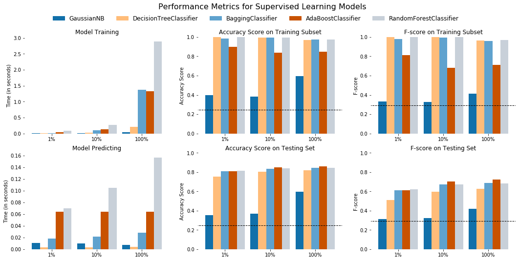
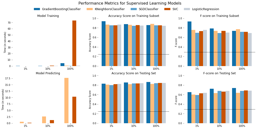
The following visualization code displays the results for the various learners.
def evaluate(results, accuracy, f1):
    """
    Visualization code to display results of various learners.

    inputs:
      - learners: a list of supervised learners
      - stats: a list of dictionaries of the statistic results from 'train_predict()'
      - accuracy: The score for the naive predictor
      - f1: The score for the naive predictor
    """

    # Create figure
    fig, ax = pl.subplots(2, 3, figsize = (18,8))

    # Constants
    bar_width = 0.175
    colors = ['#1170aa','#ffbc79','#5fa2ce', '#c85200', '#c8d0d9']

    # Super loop to plot four panels of data
    for k, learner in enumerate(results.keys()):
        for j, metric in enumerate(['train_time', 'acc_train', 'f_train', 'pred_time', 'acc_test', 'f_test']):
            for i in np.arange(3):
                # Creative plot code
                ax[j//3, j%3].bar(i+k*bar_width+0.15,
                                  results[learner][i][metric],
                                  width = bar_width,
                                  color = colors[k])
                ax[j//3, j%3].set_xticks([0.5, 1.5, 2.5])
                ax[j//3, j%3].set_xticklabels(["1%", "10%", "100%"])
                ax[j//3, j%3].set_xlim((-0.1, 3.1))
                for spine in ax[j//3, j%3].spines.values():
                    spine.set_visible(False)

    # Add unique y-labels
    ax[0, 0].set_ylabel("Time (in seconds)")
    ax[0, 1].set_ylabel("Accuracy Score")
    ax[0, 2].set_ylabel("F-score")
    ax[1, 0].set_ylabel("Time (in seconds)")
    ax[1, 1].set_ylabel("Accuracy Score")
    ax[1, 2].set_ylabel("F-score")

    # Add titles
    ax[0, 0].set_title("Model Training")
    ax[0, 1].set_title("Accuracy Score on Training Subset")
    ax[0, 2].set_title("F-score on Training Subset")
    ax[1, 0].set_title("Model Predicting")
    ax[1, 1].set_title("Accuracy Score on Testing Set")
    ax[1, 2].set_title("F-score on Testing Set")

    # Add horizontal lines for naive predictors
    ax[0, 1].axhline(y = accuracy, xmin = -0.1, xmax = 3.0, linewidth = 1, color = 'k', linestyle = 'dashed')
    ax[1, 1].axhline(y = accuracy, xmin = -0.1, xmax = 3.0, linewidth = 1, color = 'k', linestyle = 'dashed')
    ax[0, 2].axhline(y = f1, xmin = -0.1, xmax = 3.0, linewidth = 1, color = 'k', linestyle = 'dashed')
    ax[1, 2].axhline(y = f1, xmin = -0.1, xmax = 3.0, linewidth = 1, color = 'k', linestyle = 'dashed')

    # Set y-limits for score panels
    ax[0, 1].set_ylim((0, 1))
    ax[0, 2].set_ylim((0, 1))
    ax[1, 1].set_ylim((0, 1))
    ax[1, 2].set_ylim((0, 1))

    # Create patches for the legend
    patches = []
    for i, learner in enumerate(results.keys()):
        patches.append(mpatches.Patch(color = colors[i], label = learner))
    pl.legend(handles = patches, bbox_to_anchor = (-.80, 2.45), \
              loc = 'upper center', borderaxespad = 0., ncol = 5, frameon=False, fontsize = 12)

    # Aesthetics
    pl.suptitle("Performance Metrics for Supervised Learning Models", fontsize = 16, y = 1)
    pl.show()
first_five_keys = list(results.keys())[:5]
last_five_keys = list(results.keys())[5:]
first_five_results = {key: results[key] for key in first_five_keys}
last_five_results = {key: results[key] for key in last_five_keys}
evaluate(first_five_results, accuracy, fscore)
evaluate(last_five_results, accuracy, fscore)
r = (pd.DataFrame(results)
     .T
     .drop(columns=[0,1])
     .rename(columns={2:'parameters'})
     .reset_index()
     .rename(columns={'index':'model'}))
copy = r.copy()
params = pd.DataFrame()
for model in r['model']:
    param_dict = copy[copy['model']==model]['parameters'].values[0]
    p = (pd.DataFrame(param_dict,
                      [model])
         .reset_index()
         .rename(columns={'index':'model'}))
    params = (params.append(p))
params = (params
          .reset_index(drop=True))
for time in ['train_time','pred_time']:
    params[time] = params[time].round(1)
for acc in ['acc_train','acc_test','f_train','f_test']:
    params[acc] = (params[acc] * 100.).round(1)
params['acc_delta'] = params['acc_train'] - params['acc_test']
params['f_delta'] = params['f_train'] - params['f_test']
def sort_params_by(parameter, params):
    params = (params
              .sort_values([parameter],
                           ascending=False)
              .reset_index(drop=True))
    params['acc_delta'] = params['acc_train'] - params['acc_test']
    params['f_delta'] = params['f_train'] - params['f_test']
    params.index += 1
    return params
sort_params_by('acc_test', params)
| model | train_time | pred_time | acc_train | acc_test | f_train | f_test | acc_delta | f_delta | |
|---|---|---|---|---|---|---|---|---|---|
| 1 | GradientBoostingClassifier | 4.5 | 0.0 | 85.7 | 86.3 | 73.4 | 74.0 | -0.6 | -0.6 |
| 2 | AdaBoostClassifier | 1.3 | 0.1 | 85.0 | 85.8 | 71.2 | 72.5 | -0.8 | -1.3 |
| 3 | BaggingClassifier | 1.4 | 0.0 | 97.3 | 84.3 | 95.9 | 68.4 | 13.0 | 27.5 |
| 4 | RandomForestClassifier | 2.9 | 0.2 | 97.7 | 84.2 | 97.1 | 68.1 | 13.5 | 29.0 |
| 5 | SVC | 73.1 | 10.3 | 85.3 | 84.2 | 71.7 | 68.5 | 1.1 | 3.2 |
| 6 | LogisticRegression | 0.7 | 0.0 | 84.3 | 84.2 | 69.0 | 68.3 | 0.1 | 0.7 |
| 7 | SGDClassifier | 0.3 | 0.0 | 85.3 | 84.1 | 71.4 | 67.9 | 1.2 | 3.5 |
| 8 | KNeighborsClassifier | 0.5 | 17.7 | 88.3 | 82.3 | 77.2 | 63.7 | 6.0 | 13.5 |
| 9 | DecisionTreeClassifier | 0.2 | 0.0 | 97.0 | 81.9 | 96.4 | 62.8 | 15.1 | 33.6 |
| 10 | GaussianNB | 0.0 | 0.0 | 59.3 | 59.8 | 41.2 | 42.1 | -0.5 | -0.9 |
sort_params_by('f_test', params)[:1]
| model | train_time | pred_time | acc_train | acc_test | f_train | f_test | acc_delta | f_delta | |
|---|---|---|---|---|---|---|---|---|---|
| 1 | GradientBoostingClassifier | 4.5 | 0.0 | 85.7 | 86.3 | 73.4 | 74.0 | -0.6 | -0.6 |
sort_params_by('acc_train', params)[:5]
| model | train_time | pred_time | acc_train | acc_test | f_train | f_test | acc_delta | f_delta | |
|---|---|---|---|---|---|---|---|---|---|
| 1 | RandomForestClassifier | 2.9 | 0.2 | 97.7 | 84.2 | 97.1 | 68.1 | 13.5 | 29.0 |
| 2 | BaggingClassifier | 1.4 | 0.0 | 97.3 | 84.3 | 95.9 | 68.4 | 13.0 | 27.5 |
| 3 | DecisionTreeClassifier | 0.2 | 0.0 | 97.0 | 81.9 | 96.4 | 62.8 | 15.1 | 33.6 |
| 4 | KNeighborsClassifier | 0.5 | 17.7 | 88.3 | 82.3 | 77.2 | 63.7 | 6.0 | 13.5 |
| 5 | GradientBoostingClassifier | 4.5 | 0.0 | 85.7 | 86.3 | 73.4 | 74.0 | -0.6 | -0.6 |
sort_params_by('f_train', params)[:5]
| model | train_time | pred_time | acc_train | acc_test | f_train | f_test | acc_delta | f_delta | |
|---|---|---|---|---|---|---|---|---|---|
| 1 | RandomForestClassifier | 2.9 | 0.2 | 97.7 | 84.2 | 97.1 | 68.1 | 13.5 | 29.0 |
| 2 | DecisionTreeClassifier | 0.2 | 0.0 | 97.0 | 81.9 | 96.4 | 62.8 | 15.1 | 33.6 |
| 3 | BaggingClassifier | 1.4 | 0.0 | 97.3 | 84.3 | 95.9 | 68.4 | 13.0 | 27.5 |
| 4 | KNeighborsClassifier | 0.5 | 17.7 | 88.3 | 82.3 | 77.2 | 63.7 | 6.0 | 13.5 |
| 5 | GradientBoostingClassifier | 4.5 | 0.0 | 85.7 | 86.3 | 73.4 | 74.0 | -0.6 | -0.6 |
Select Top Model and Discuss Results
As shown in the table and charts above, the top-performing algorithm is the GradientBoostingClassifier.
- It has the highest accuracy and f-score on the test set.
- It has the fifth highest accuracy and f-score on the training set, but all models that outperformed it on these two metrics overfit the data.
- The evidence of the overfit is the large deltas these models have between their performance on the training set and testing set. These deltas range from 6 percentage points on the low end to 33.6 percentage points on the high end. The
GradientBoostingClassifier, on the other hand, actually performs slightly better on the test set than on the training set.
- The evidence of the overfit is the large deltas these models have between their performance on the training set and testing set. These deltas range from 6 percentage points on the low end to 33.6 percentage points on the high end. The
- The training and prediction time both only take single-digits seconds to complete. The
SVCclassifier took the longest to train, by far, while theKNeighborsClassifiertook the longest to predict. - As an ensemble learner that is suited to classification, the
GradientBoostingClassifieris well-suited to this dataset.
Model Description 1, 2, 3
Sklearn’s GradientBoostingClassifier is one specific implementation of Gradient Boosting. GB is a group of algorithms that are referred to as ensemble learners because they involve creating groups, or ensembles, of many other “weak learners” which vote on the output of the overall group. Weak learners is a term used to describe a simple model that is able to correctly predict more often than a random choice, but which are not powerful enough to be used as a predictor on their own. These weak learners are generally decision trees. These weak learners are sometimes referred to as decision stumps because their structure is often very limited. Often, they are a single decision node, for example.
Gradient Boosting begins by fitting a single weak learner on the dataset. New, additional weak learners are iteratively added to the ensemble. Those new learners are specifically trained to reduce error between the model’s predictions and the true labels in the dataset. By “focusing on the weak spots,” the performance of the overall model is improved with each training iteration. Once the model reaches a certain performance and/or complexity, the model training is considered completed and no additional learners are added. The trained model makes predictions by having the ensembled learners vote on each prediction the model makes.