Analyzing the Stroop Effect using T-Tests
Table of Contents
- Intro
- Identification of Variables
- Select Statistical Test
- Establish Hypotheses
- Calculate Descriptive Statistics to Build Intuition
- Visualize the Data
- Perform the Statistical Test
Introduction
The Stroop effect is a psychological phenomenon that impacts the reaction time required for certain cognitive tasks. The most common manifestation of the effect occurs during the performance of a “Stroop test,” during which participants are asked to name the font color a list of colors are printed in.
There are two types of lists the participants read from. “Congruent” lists are those where the written color and the font color are the same. “Incongruent” lists are those where the written color is different from the font color.
Congruent:
Blue Red Green Red Blue Blue Green
Incongruent:
Blue Red Green Red Blue Blue Green
The idea is that it takes participants significantly longer to state the color each word is written in for the incongruent list than for the congruent list.
Identification of Variables
Independent variable: which list is shown to the participant.
Dependent variable: the amount of time it takes the participant to name the ink colors for each list.
Select Statistical Test
Since the goal of this anlysis is to infer something about the population from limited samples, the hypothesis will be written in terms of the population mean, $\mu$.
The appropriate statistical test to perform is the “Dependent Samples T Test.” This test is also known as the “Paired Samples T Test.” This is the appropriate test because the data involve two measurements performed on the same person under different conditions, and contains no information about the population.
Establish Hypotheses
Since the goal is to prove the presence of the stroop effect, the appropriate structure for the set of hypotheses is to make the implicit assumption that the stroop effect does not exist.
That is, the alternative hypothesis is that the mean difference between the time required to read the incongruent and congruent lists is greater than zero. Then, the null hypothesis (initially assumed to be correct) is that the mean difference between the time required to read the incongruent and congruent lists is zero.
Recall that congruent means the ink color is the same as the written color, whereas incongruent means the ink color is different from the written color.
Written algebraically, the foregoing becomes the following…
$$H_0: \mu_{diff} = 0$$ $$H_A: \mu_{diff}> 0$$
where, $\mu_{diff}$ is defined as the average of the pairwise differences, $x_{diff}$:
$$x_{diff} = x_{incongruent}-x_{congruent}$$
The fact that the samples are dependent is why also why the hypotheses are written in terms of the mean of differences, rather than the difference of means, although those approaches are only subtely different. Rarely would they produce different results.
Calculate Descriptive Statistics to Build Intuition
import pandas as pd
import matplotlib.pyplot as plt
from scipy import stats
%matplotlib inline

df = pd.read_csv('data/stroopdata.csv')
df.shape
(24, 2)
24 participants completed the study.
df['difference'] = df['Incongruent'] - df['Congruent']
df.head()
| Congruent | Incongruent | difference | |
|---|---|---|---|
| 0 | 12.079 | 19.278 | 7.199 |
| 1 | 16.791 | 18.741 | 1.950 |
| 2 | 9.564 | 21.214 | 11.650 |
| 3 | 8.630 | 15.687 | 7.057 |
| 4 | 14.669 | 22.803 | 8.134 |
cong_mean =   df.Congruent.mean()
cong_std =    df.Congruent.std()
incong_mean = df.Incongruent.mean()
incong_std =  df.Incongruent.std()
diff_mean =   df.difference.mean()
diff_std =    df.difference.std()
diff_min =    df.difference.min()

print('  Congruent data -    mean :  {:.1f}'.format(cong_mean))
print('  Congruent data - std dev :   {:.1f}'.format(cong_std))
print('\r')
print('Incongruent data -    mean :  {:.1f}'.format(incong_mean))
print('Incongruent data - std dev :   {:.1f}'.format(incong_std))
print('\r')
print(' Difference data -    mean :   {:.1f}'.format(diff_mean))
print(' Difference data - std dev :   {:.1f}'.format(diff_std))
print('\r')
print(' Difference data -     min :   {:.1f}'.format(diff_min))
  Congruent data -    mean :  14.1
  Congruent data - std dev :   3.6

Incongruent data -    mean :  22.0
Incongruent data - std dev :   4.8

 Difference data -    mean :   8.0
 Difference data - std dev :   4.9

 Difference data -     min :   1.9
The descriptive statistics above imply that the null will be rejected, for two reasons:
- A positive mean difference, with magnitude of nearly twice the standard deviation.
- There are no negative values in the difference data, as evidenced by the minimum value.
Visualize the Data
def print_hists():
    fig, axs = plt.subplots(1, 3, figsize=(16,4))
    bins = range(0,35,5)
    colors = ['lightblue', 'pink', 'lightgreen']
    means = [cong_mean, incong_mean, diff_mean]

    axs[0].hist(df.Congruent, label='Congruent',
                color=colors[0], bins=bins);

    axs[1].hist(df.Incongruent, label='Incongruent',
                color=colors[1], bins=bins);

    axs[2].hist(df.difference, label='Difference',
                color=colors[2], bins=bins);

    for i, ax in enumerate(axs):
        ax.axvline(means[i], color='black');
        ax.legend();

        for label in ['top', 'bottom', 'right', 'left']:
            ax.spines[label].set_visible(False)
def print_boxplots():
    fig, ax = plt.subplots(1, 1, figsize=(16,6))
    colors = ['lightblue', 'pink', 'lightgreen']

    bp = ax.boxplot([df.Congruent, df.Incongruent, df.difference],
                    labels = ['Congruent', 'Incongruent', 'Difference'],
                    patch_artist = True);

    for label in ['top', 'right', 'left']:
        ax.spines[label].set_visible(False)

    for i, box in enumerate(bp['boxes']):
        box.set(color = colors[i], linewidth = 3)

    for i, whisker in enumerate(bp['whiskers']):
        whisker.set(color = colors[i//2], linewidth = 3)

    for i, cap in enumerate(bp['caps']):
        cap.set(color = colors[i//2], linewidth = 3)

    for i, flier in enumerate(bp['caps']):
        flier.set(color = colors[i//2], linewidth = 3)
print_hists()
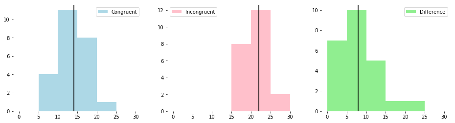
The three histograms above are plotted on a common x-axis. The values of the incongruent data appear to be generally higher than the congruent data.
print_boxplots()
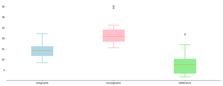
The box plots, above, provide another way to visualize the information in the histograms. Both types of plots appear to provide further indication of the presence of the Stroop effect. The null hypothesis is expected to be rejected based on the distributions of the data shown above.
Perform the Statistical Test
To perform the statistical test, I calculate the “p-value,” which is the strength of evidence in support of the null hypothesis.
As a standard of comparison for the p-value, I adopt the standard $\alpha$, or “Significance Level,” of 0.05. This is the probability of rejecting the null hypothesis when it is actually true. To arrive at a p value for this set of data, I calculate the t-statistic, which in turn requires the standard error:
$$SE = \frac{\sigma}{n^\frac{1}{2}}$$
where $\sigma$ is the standard deviation of the sample, and $n$ is the number of samples.
The t-statistic is calculated as:
$$t_{stat} = \frac{\mu_{diff}}{SE}$$
where $\mu_{diff}$ is the standard deviation of the differences between the congruent and incongruent test durations for each participant.
Finally, the p-value is calculated using the Cumulative Distribution Function, which requires as inputs the $t_{stat}$ and degrees of freedom. The degrees of freedom are calculated as $n-1$, where $n$, as above, is the number of samples.
$$p_{value} = 1-CDF(t_{stat}, n-1)$$
diff_standard_error = diff_std / (df.shape[0]**0.5)
t_stat = diff_mean / diff_standard_error
p_value = 1-stats.t.cdf(t_stat, df.shape[0]-1)

print('Difference standard error = {:.3f}'.format(diff_standard_error))
print('     T-stat for test data = {:.2f}'.format(t_stat))
print(' P-value for given t-stat = {:.9f}'.format(p_value))
Difference standard error = 0.993
     T-stat for test data = 8.02
 P-value for given t-stat = 0.000000021
The p-value, shown above, is the probability of rejecting the null hypothesis when it is actually true. Another value, called the “Confidence Level,” is 1 minus $\alpha$, expressed as a percentage. For a significance level of 0.05, the confidence level is 95%.
The T-stat for our test data is 8.02, which, for 23 degrees of freedom, corresponds to a P-value much less than 0.05. Since the P-value is less than the significance level, I reject the null hypothesis. The conclusion is that the alternative hypothesis is true, and that the Stroop effect has had a statistically-significant impact.
Having taken this particular test myself before, I am not surprised by the results. Even with significant concentration it is difficult to quickly say the ink color a word is written in when that word itself spells out a color.