Random Projection and ICA
Random Projection
Random Projection is a powerful dimensionality reduction technique that is computationally more efficient than PCA. The quality of the projection is decreased, however.
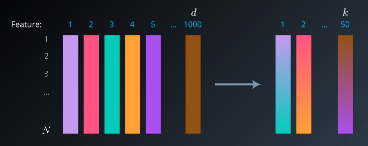
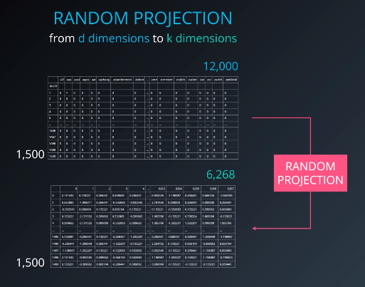
Random Projections takes a large dataset and produces a transformation of it that is in a much smaller number of columns.
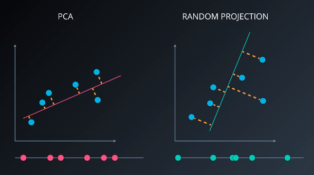
Conceptually, Random Projections differs from PCA in a simple way. Where PCA calculates the vector or direction that maximizes the variance so loses the least amount of information during the projection, Random Projection simply picks any vector and then performs the projection. This works very well in high dimensional spaces and is very computationally efficient.
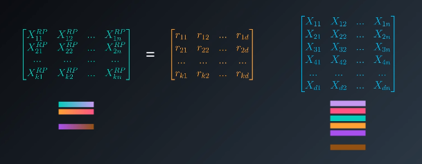
The basic premise is that it is possible to reduce the number of dimensions in a dataset by multiplying the dataset by a random matrix.
$$X^{RP}_{kxN} = R_{kxd} X_{dxN}$$
The theoretical underpinning is something called the Johnson-Lindenstrauss lemma: “A dataset of N points in high-dimensional Euclideanspace can be mapped down to a space in much lower dimension in a way that preserves the distance between the points to a large degree.”
The algorithms work by only allowing a certain maximum deviation in the distances. This maximum deviation is a value, $\epsilon$, that is a parameter of the algorithm. That value preserves the distances of every other point.
In Sklearn, SparseRandomProjection is more performant than GaussianRandomProjection
from sklearn import random_projection

rp = random_projection.SparseRandomProjection()

new_x = rp.fit_transform(X)
Independent Component Analysis
Independent Component Analysis, ICA, is method similar to Principle Component Analysis, PCA, and random projection in that it takes a set of features and produces a different set that is useful in some way. It is different in that where PCA attempts to maximize variance, ICA assumes that the features are mixtures of independent sources, which it tries to isolate.
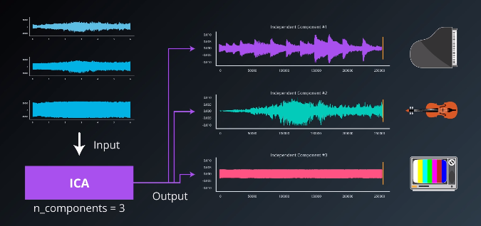
The specific problem ICA solves is called the “blind source problem.” A classic example is the “cocktail party problem.” The cocktail party is a somewhat contrived situation in which three people are at a cocktail party where three different sources of sound are playing simultaneously: a piano, a violin, and a television that is generating white noise. All record the sounds.

Imagine one friend is seated closest to the piano, another, the violin, and the third is closest to the television. The volume levels of the different sound sources will be different.

Given each of those three recordings, ICA would be able to extract the original three sound components.
To unpack how ICA works in more depth, we need to introduce some notation. Let the $X$ denote the datasets, or recordings. Let $A$ be the amplitudes of the various sources, or the “mixing matrix”. And, let $S$ be the actual source audio we hope to reconstruct.
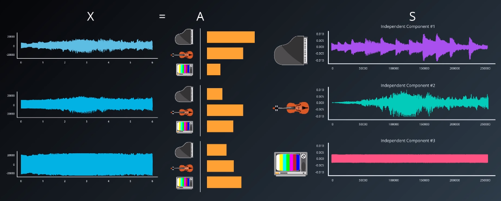
Then, the dataset is given by $X=AS$. The source audio can be reconstructed by taking $S=A^{-1} X$. The ICA algorithm is a means of approximating the “un-mixing” matrix, $A^{-1}$. The more detailed mathematics behind ICA are documented in this paper. ICA relies on the Central Limit Theorem, and, in particular, makes the following assumptions:
- The components are statistically independent,
- The components must have non-Gaussian distributions.
A final note is that ICA needs as many observations (microphones) as the original signals we are trying to separate.
from sklearn.decomposition import FastICA

# Each 'signal' variable is an array. For example, an audio waveform
X = list(zip(signal_1, signal_2, signal_3))

ica = FastICA(n_components=3)

components = ica.fit_transform(X)

# components now contains the independent components retrieved via ICA
ICA is widely-used in medical imaging, specifically to transform EEG scan data to do blind source separation. This paper documents the use case. The raw EEG scan includes mixtures of many brain waves, whereas the ICA transformed data isolates the independent waveforms the brain generates. ICA is used for similar purposes in MRIs.
There have also been attempts to use ICA on financial data, including stock prices, though the economy is such a complex machine that the approach has had only limited success.