Hierarchical Clustering
In this notebook, I use sklearn to conduct hierarchical clustering on the Iris dataset which contains 4 dimensions/attributes and 150 samples. Each sample is labeled as one of the three type of Iris flowers.
Load the Iris Dataset
from sklearn import datasets

iris = datasets.load_iris()
iris.data contains the features; iris.target contains the labels.
iris.data[45:55]
array([[4.8, 3. , 1.4, 0.3],
       [5.1, 3.8, 1.6, 0.2],
       [4.6, 3.2, 1.4, 0.2],
       [5.3, 3.7, 1.5, 0.2],
       [5. , 3.3, 1.4, 0.2],
       [7. , 3.2, 4.7, 1.4],
       [6.4, 3.2, 4.5, 1.5],
       [6.9, 3.1, 4.9, 1.5],
       [5.5, 2.3, 4. , 1.3],
       [6.5, 2.8, 4.6, 1.5]])
iris.target[45:55]
array([0, 0, 0, 0, 0, 1, 1, 1, 1, 1])
import pandas as pd

df = (pd.DataFrame(iris.data))
df.describe()
| 0 | 1 | 2 | 3 | |
|---|---|---|---|---|
| count | 150.000000 | 150.000000 | 150.000000 | 150.000000 |
| mean | 5.843333 | 3.057333 | 3.758000 | 1.199333 |
| std | 0.828066 | 0.435866 | 1.765298 | 0.762238 |
| min | 4.300000 | 2.000000 | 1.000000 | 0.100000 |
| 25% | 5.100000 | 2.800000 | 1.600000 | 0.300000 |
| 50% | 5.800000 | 3.000000 | 4.350000 | 1.300000 |
| 75% | 6.400000 | 3.300000 | 5.100000 | 1.800000 |
| max | 7.900000 | 4.400000 | 6.900000 | 2.500000 |
Perform Clustering
Use sklearn’s AgglomerativeClustering to conduct the heirarchical clustering
Ward is the default linkage algorithm
from sklearn.cluster import AgglomerativeClustering

ward = AgglomerativeClustering(n_clusters=3)
ward_pred = ward.fit_predict(iris.data)
Also use: complete, average, single
complete = AgglomerativeClustering(n_clusters=3,
                                   linkage='complete')
complete_pred = complete.fit_predict(iris.data)
single = AgglomerativeClustering(n_clusters=3,
                                 linkage='single')
single_pred = single.fit_predict(iris.data)
average = AgglomerativeClustering(n_clusters=3,
                                  linkage='average')
average_pred = average.fit_predict(iris.data)
To determine which clustering result best matches the original labels, use adjusted_rand_score, an external cluster validation index that results in a score between -1 and 1. 1 indicates the clsuters are identical (regardless of specific label).
from sklearn.metrics import adjusted_rand_score
ward_ar_score = adjusted_rand_score(iris.target, ward_pred)
complete_ar_score = adjusted_rand_score(iris.target, complete_pred)
single_ar_score = adjusted_rand_score(iris.target, single_pred)
average_ar_score = adjusted_rand_score(iris.target, average_pred)
print("Ward       {:2.1%}".format(ward_ar_score),
      "\nComplete   {:2.1%}".format(complete_ar_score),
      "\nAverage    {:2.1%}".format(average_ar_score),
      "\nSingle     {:2.1%}".format(single_ar_score))
Ward       73.1%
Complete   64.2%
Average    75.9%
Single     56.4%
The Effect of Normalization on Clustering
The fourth column has smaller values than the rest of the columns, so its variance currently counts for less in the clustering process. By normalizing the dataset so that each dimension lies between 0 and 1, they will have equal weight. This done by subtracting the minimum from each column then dividing the difference by the range.
df.describe()
| 0 | 1 | 2 | 3 | |
|---|---|---|---|---|
| count | 150.000000 | 150.000000 | 150.000000 | 150.000000 |
| mean | 5.843333 | 3.057333 | 3.758000 | 1.199333 |
| std | 0.828066 | 0.435866 | 1.765298 | 0.762238 |
| min | 4.300000 | 2.000000 | 1.000000 | 0.100000 |
| 25% | 5.100000 | 2.800000 | 1.600000 | 0.300000 |
| 50% | 5.800000 | 3.000000 | 4.350000 | 1.300000 |
| 75% | 6.400000 | 3.300000 | 5.100000 | 1.800000 |
| max | 7.900000 | 4.400000 | 6.900000 | 2.500000 |
from sklearn import preprocessing

normalized_X = preprocessing.normalize(iris.data)
pd.DataFrame(normalized_X).describe()
| 0 | 1 | 2 | 3 | |
|---|---|---|---|---|
| count | 150.000000 | 150.000000 | 150.000000 | 150.000000 |
| mean | 0.751400 | 0.405174 | 0.454784 | 0.141071 |
| std | 0.044368 | 0.105624 | 0.159986 | 0.077977 |
| min | 0.653877 | 0.238392 | 0.167836 | 0.014727 |
| 25% | 0.715261 | 0.326738 | 0.250925 | 0.048734 |
| 50% | 0.754883 | 0.354371 | 0.536367 | 0.164148 |
| 75% | 0.786912 | 0.527627 | 0.580025 | 0.197532 |
| max | 0.860939 | 0.607125 | 0.636981 | 0.280419 |
ward = AgglomerativeClustering(n_clusters=3)
ward_pred = ward.fit_predict(normalized_X)

complete = AgglomerativeClustering(n_clusters=3, linkage="complete")
complete_pred = complete.fit_predict(normalized_X)

avg = AgglomerativeClustering(n_clusters=3, linkage="average")
avg_pred = avg.fit_predict(normalized_X)

single = AgglomerativeClustering(n_clusters=3, linkage="single")
single_pred = single.fit_predict(normalized_X)

n_ward_ar_score = adjusted_rand_score(iris.target, ward_pred)
n_complete_ar_score = adjusted_rand_score(iris.target, complete_pred)
n_avg_ar_score = adjusted_rand_score(iris.target, avg_pred)
n_single_ar_score = adjusted_rand_score(iris.target, single_pred)

print('          Unnormalized   Normalized',
      "\nWard      {:12.1%}   {:10.1%}".format(ward_ar_score, n_ward_ar_score),
      "\nComplete  {:12.1%}   {:10.1%}".format(complete_ar_score, n_complete_ar_score),
      "\nAverage   {:12.1%}   {:10.1%}".format(average_ar_score, n_avg_ar_score),
      "\nSingle    {:12.1%}   {:10.1%}".format(single_ar_score, n_single_ar_score))
          Unnormalized   Normalized
Ward             73.1%        88.6%
Complete         64.2%        64.4%
Average          75.9%        55.8%
Single           56.4%        55.8%
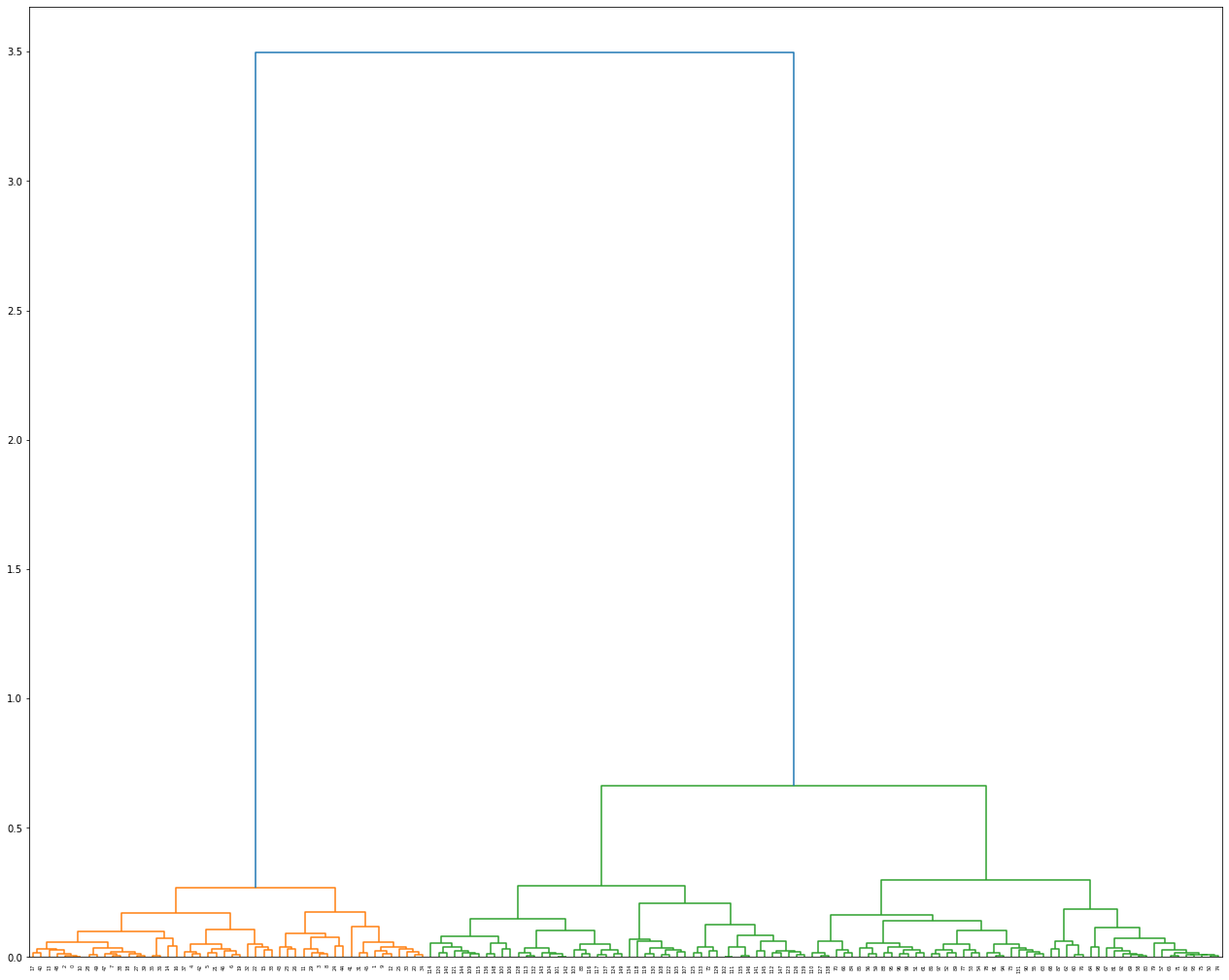
Dendrogram visualization with scipy
Visualize the highest scoring clustering result. To do this, use Scipy’s linkage function to perform the clustering again. This will enable us to obtain the linkage matrix it will use later to visualize the hierarchy.
from scipy.cluster.hierarchy import linkage

linkage_type = 'ward'

linkage_matrix = linkage(normalized_X, linkage_type)
from scipy.cluster.hierarchy import dendrogram
import matplotlib.pyplot as plt
plt.figure(figsize=(22,18))

# plot using 'dendrogram()'
dendrogram(linkage_matrix)

plt.show()
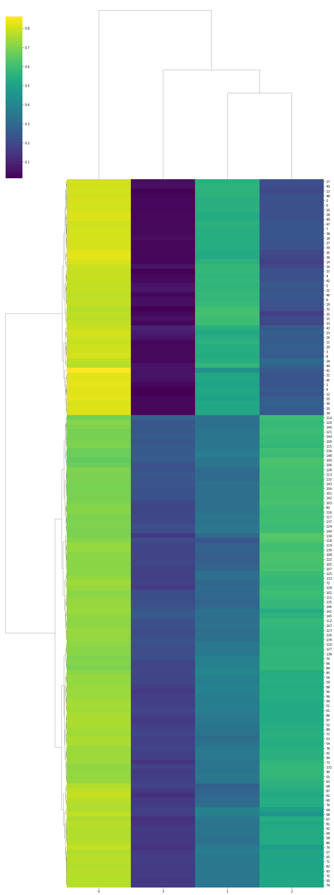
Visualization with Seaborn’s clustermap
The seaborn plotting library for python can plot a clustermap, which is a detailed dendrogram which also visualizes the dataset in more detail. It conducts the clustering as well. So, you only need to pass it the dataset and the linkage type, and it will use scipy internally to conduct the clustering.
import seaborn as sns

sns.clustermap(normalized_X,
               figsize=(15,40),
               method=linkage_type,
               cmap='viridis')
plt.show()