Gaussian Mixture Model Examples
1. KMeans versus GMM on a Generated Dataset
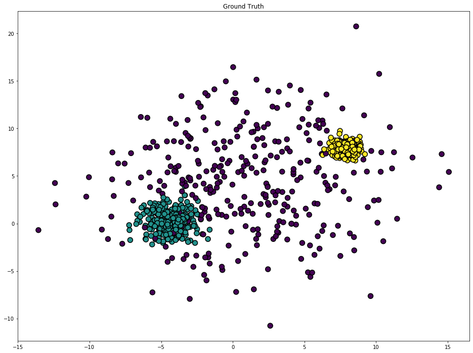
Use sklearn’s make_blobs function to create a dataset of Gaussian blobs.
import numpy as np
import matplotlib.pyplot as plt
from sklearn import cluster, datasets, mixture

%matplotlib inline

n_samples = 1000

varied = datasets.make_blobs(n_samples=n_samples,
                             cluster_std=[5, 1, 0.5],
                             random_state=3)
X, y = varied[0], varied[1]

plt.figure(figsize=(16,12))
plt.scatter(X[:,0], X[:,1],
            c=y, edgecolor='black', lw=1.5,
            s=100, cmap=plt.get_cmap('viridis'))
plt.title('Ground Truth')
plt.show()
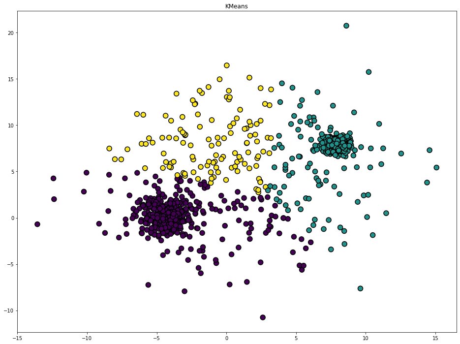
KMeans
from sklearn.cluster import KMeans

kmeans = KMeans(n_clusters=3)
pred = kmeans.fit_predict(X)

plt.figure( figsize=(16,12))
plt.scatter(X[:,0], X[:,1],
            c=pred, edgecolor='black', lw=1.5,
            s=100, cmap=plt.get_cmap('viridis'))
plt.title('KMeans')
plt.show()
GuassianMixture
from sklearn.mixture import GaussianMixture

gmm = GaussianMixture(n_components=3).fit(X)
gmm = gmm.fit(X)
pred_gmm = gmm.predict(X)

plt.figure( figsize=(16,12))
plt.scatter(X[:,0], X[:,1], c=pred_gmm, edgecolor='black', lw=1.5, s=100, cmap=plt.get_cmap('viridis'))
plt.show()
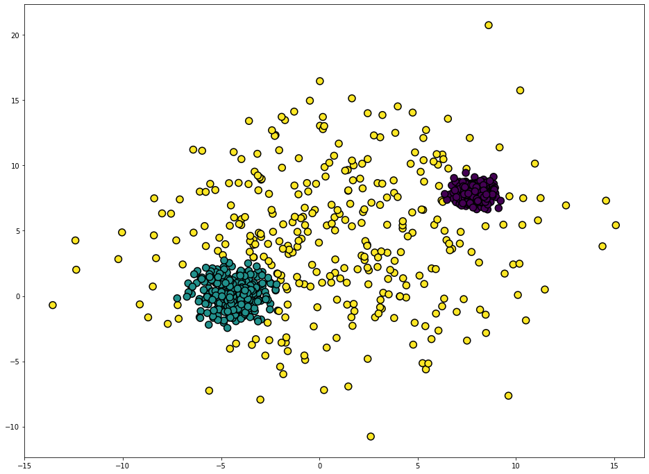
GaussianMixture clearly outperforms Kmeans on this dataset. This is expected since make_blobs creates Gaussian blobs.
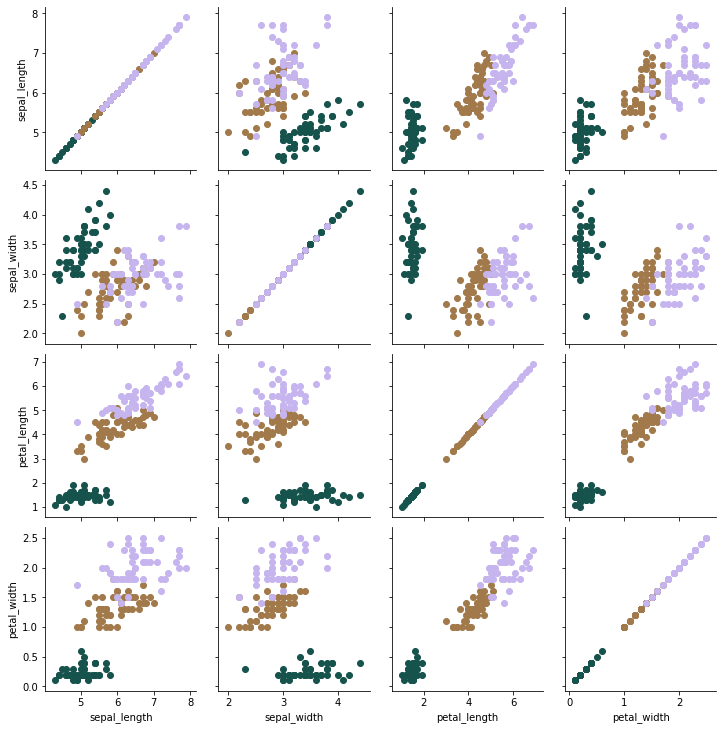
2. KMeans versus GMM on the Iris Dataset
For the second example, use the Iris dataset. The Iris Dataset is great for this purpose since it is likely the data is normally-distributed.
import seaborn as sns

iris = sns.load_dataset("iris")

iris.info()
iris.head()
<class 'pandas.core.frame.DataFrame'>
RangeIndex: 150 entries, 0 to 149
Data columns (total 5 columns):
 #   Column        Non-Null Count  Dtype
---  ------        --------------  -----
 0   sepal_length  150 non-null    float64
 1   sepal_width   150 non-null    float64
 2   petal_length  150 non-null    float64
 3   petal_width   150 non-null    float64
 4   species       150 non-null    object
dtypes: float64(4), object(1)
memory usage: 6.0+ KB
| sepal_length | sepal_width | petal_length | petal_width | species | |
|---|---|---|---|---|---|
| 0 | 5.1 | 3.5 | 1.4 | 0.2 | setosa |
| 1 | 4.9 | 3.0 | 1.4 | 0.2 | setosa |
| 2 | 4.7 | 3.2 | 1.3 | 0.2 | setosa |
| 3 | 4.6 | 3.1 | 1.5 | 0.2 | setosa |
| 4 | 5.0 | 3.6 | 1.4 | 0.2 | setosa |
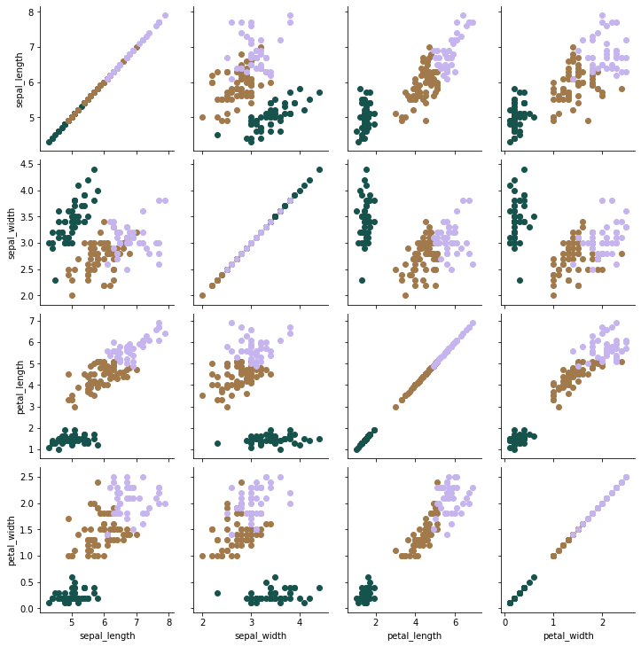
There are several ways to visualize a dataset with four dimensions, such as:
Use PairGrid since it does not distort the dataset. It simply plots every pair of features against each other in a subplot.
g = sns.PairGrid(iris, hue="species",
                 palette=sns.color_palette("cubehelix", 3),
                 vars=['sepal_length','sepal_width',
                       'petal_length','petal_width'])
g.map(plt.scatter)
plt.show()
kmeans_iris = KMeans(n_clusters=3)
pred_kmeans_iris = kmeans_iris.fit_predict(iris[['sepal_length',
                                                 'sepal_width',
                                                 'petal_length',
                                                 'petal_width']])

iris['kmeans_pred'] = pred_kmeans_iris

g = sns.PairGrid(iris, hue="kmeans_pred",
                 palette=sns.color_palette("cubehelix", 3),
                 vars=['sepal_length','sepal_width',
                       'petal_length','petal_width'])
g.map(plt.scatter)
plt.show()
Visual inspection is no longer useful since we are working with multiple dimensions. Instead, use the adjusted Rand score which generates a score betwen -1 and 1, where an exact match would be scored as a 1.
from sklearn.metrics import adjusted_rand_score

iris_kmeans_score = adjusted_rand_score(iris['species'],
                                        iris['kmeans_pred'])
round(iris_kmeans_score,3)
0.73
Now, try with Gaussian Mixture models.
gmm_iris = GaussianMixture(n_components=3).fit(iris[['sepal_length',
                                                     'sepal_width',
                                                     'petal_length',
                                                     'petal_width']])
pred_gmm_iris = gmm_iris.predict(iris[['sepal_length',
                                       'sepal_width',
                                       'petal_length',
                                       'petal_width']])

iris['gmm_pred'] = pred_gmm_iris

iris_gmm_score = adjusted_rand_score(iris['species'],
                                     iris['gmm_pred'])

round(iris_gmm_score,3)
0.904
The Gaussian Mixture model outperforms KMeans according to the ARI scores.