Support Vector Machines
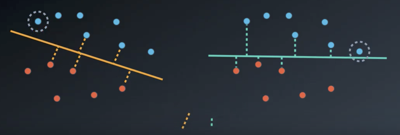
Support vector machines are a powerful algorithm for classification. They aim to not only separate the data, but also to find the best possible boundary between the classes. The best possible boundary is the one that maintains the largest possible distance from the points.

In the image above, the yellow line does a better job separating the two classes than the green line does. This becomes obvious when comparing the distance from each of the two circled points in the image below to each respective line. The yellow line maintains a greater distance from the nearest point to the line, so it is the better classifier.
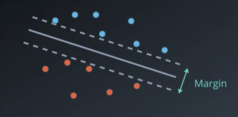
Maximize the Margin
More technically, what SVMs aim to do is maximize the margin, or the distance between the two oppositely-classified points that are closes to classification boundary.
Minimize the Error
In more complicated situations where the data are not linearly separable, such as in the image below, the best classifiers also minimize the error. The errors are all the points that are in the margin or on the wrong side of the classification boundary. These are circled yellow in the image below.

The best classifiers minimize the total error, where
$$Error = Classification\ Error + Margin\ Error$$
This total error is minimized using gradient descent.
Classification Error
The actual error calculation is like taking the sum of the distances of the misclassified points to the boundary. The optimal $w$ and $b$ for the line are found by minimizing the error using gradient descent. This is very similar to the way the perceptron algorithm works.
In the example above, $Classification\ Error=1.5+3.5+0.5+2+3+0.3=10.8$.
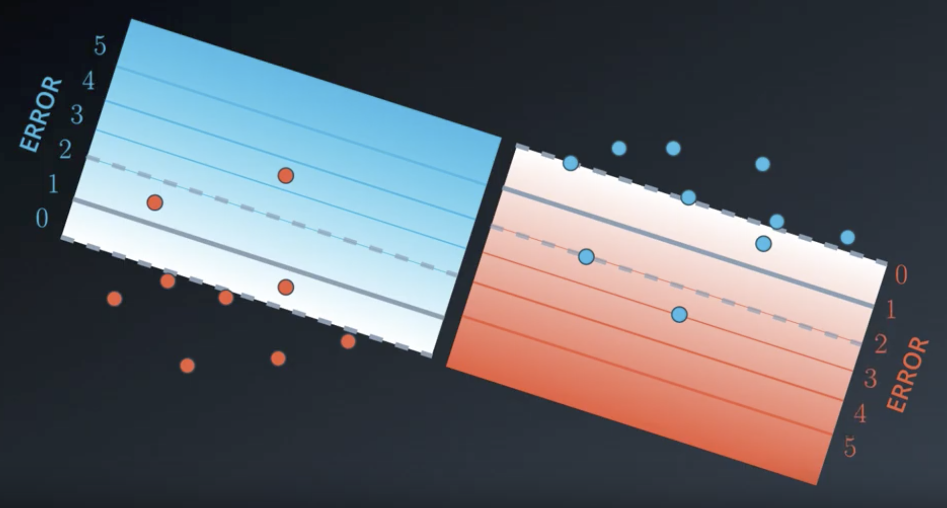
Margin error
In the image below, the models on the left and right have large and small margins, respectively.
The formulae for margin and error follow. Note that a large margin results in small error and a small margin results in a large error.
$$Margin = \frac{2}{|W|}$$
$$Error = |W|^2$$
Margin Error Examples
Two examples of high and low margin support vector machines are shown below. Both are lines of the form $w_1 x_1 + w_2 x_2 + b = 0$.
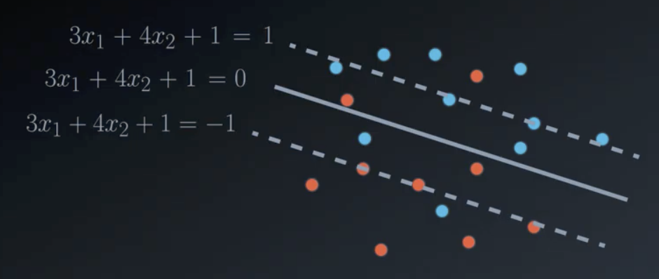
$$W = (3, 4), b = 1\ \rightarrow\ 3x_1 + 4x_2+1=0$$
$$Error = |W|^2 = 3^2 + 4^2 = 25$$
$$Margin = \frac{2}{|W|} = \frac{2}{5}$$

$$W = (6, 8), b = 2\ \rightarrow\ 6x_1 + 8x_2+2=0$$
$$Error = |W|^2 = 6^2 + 8^2 = 100$$
$$Margin = \frac{2}{|W|} = \frac{2}{10}$$
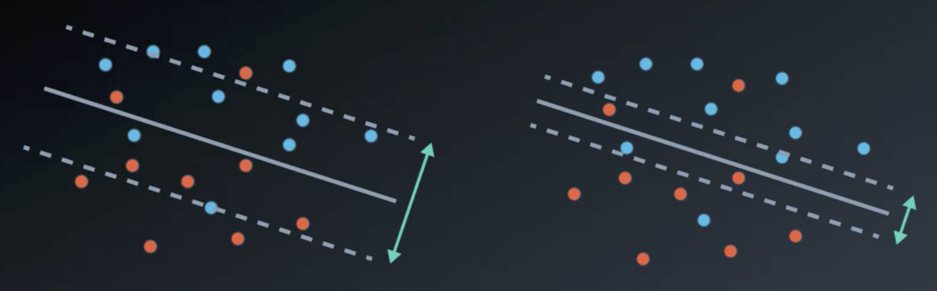
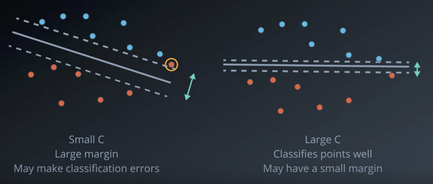
The C Parameter
Depending upon the situation, either of the following classifiers could be the more appropriate one to use.

SVMs have this flexibility built in as the C parameter, which is a variable that is multiplied by the classification error when determining the classifier’s total error.
$$Error = C \times Classification\ Error + Margin\ Error$$
- Large C: Focus is on classifying points
- Small C: Focus on large margin
Values for C can range between 0 and infinity. But, depending on the dataset, the algorithm may not converge at all. With large C values, it may not be possible to separate the data with the small number of errors allotted with large values of C.
Polynomial Kernel
1-D Example
Consider a 1-dimensional dataset like that shown below. The points are not separable by a line.

If, however, we project the points on the line into a second dimension as shown in the image below, then they become separable by a line.

Using the two equations, $y=x^2$ and $y=4$, we can solve for x: $x^2=4$. Then, we can project the solution to this equation, $x \in (-2,2)$ back onto the original line.

Notice these two lines split the data very well. This is known as the kernel trick. These are widely used in support vector machines and other algorithms in machine learning.
2-D Example
The example below is in 2 dimensions and, as in the last example, is not linearly separable. There are two ways of splitting the data: a circle and moving the points into a higher dimension.


In the first case, the linearity of the boundary is sacrificed. In the second case, the dimensionality of the data is sacrificed.
These methods are actually the same. Both rely on the equation $x^2 + y^2 = z$. For the blue points, $x^2 + y^2 = 2$. For the red points, $x^2 + y^2 = 18$. So, the circle $x^2 + y^2 = 10$ cleanly separates the points.

If we consider the separating circle as not a circle but a paraboloid that intersects the plane $z=10$, then it becomes clear how the two methods are actually the same.

Summary
Lets assume we are given a 2-dimensional set of points that cannot be linearly separable. Using the polynomial kernel in an SVM entails converting the two dimensions, $x,y$ into a 5-dimensional space, $x,y,x^2,xy,y^2)$. For example, the 2-dimensional point $(2,3)$ would be converted to the five dimensional point $(2,3,4,6,9)$.
In the 2-dimensional space, the only possible boundaries are lines. In this higher dimensional space, it may be possible to separate the data with a 4-dimensional hyperplane. In addition to lines, we can also use circles, hyperbolas, parabolas, etc.
Following the conversion, the algorithm works exactly as before. It is also possible to convert the data to an even higher dimensional space. For example, a degree 3 polynomial would have all the degree 2 monomials available as well as to the the following: $x^3, x^2y, xy^2, x^3$.
RBF Kernel (Radial Basis Functions)
By far, the most popular type of kernel is the RBF kernel. It is a density-based approach that looks at the closeness of points to one another. It allows the user the opportunity to classify points that seem hard to separate in any space.
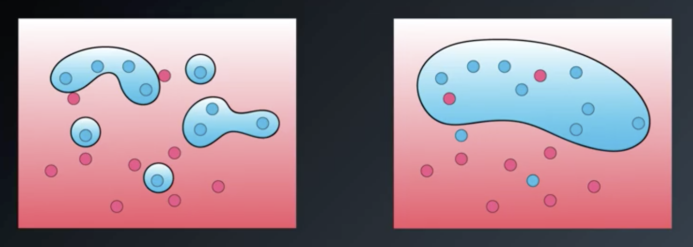
Consider again a situation where the data we have is not linearly separable.

Radial Basis Functions are a different type of kernel trick. They involve transforming the data into a higher dimensional space where the data is separable.

After the conversion and separation, the separating line is converted back down into the lower-dimensional space.

Constructing the function that facilitate this conversion entails building individual functions, each with a peak above every point.

Then, the functions above one of the two categories are inverted and the individual functions are summed up into a single separating functions.

The points are converted onto that RBF, and the separating line drawn. Finally, the function is converted back into the lower-dimensional space.

In addition to inverting the individual functions, we can also multiply them by arbitrary scalar values. So, for example, we could be given the green, yellow, and brown functions in the image below. At each of the points, consider that the functions have the values indicated in the image.
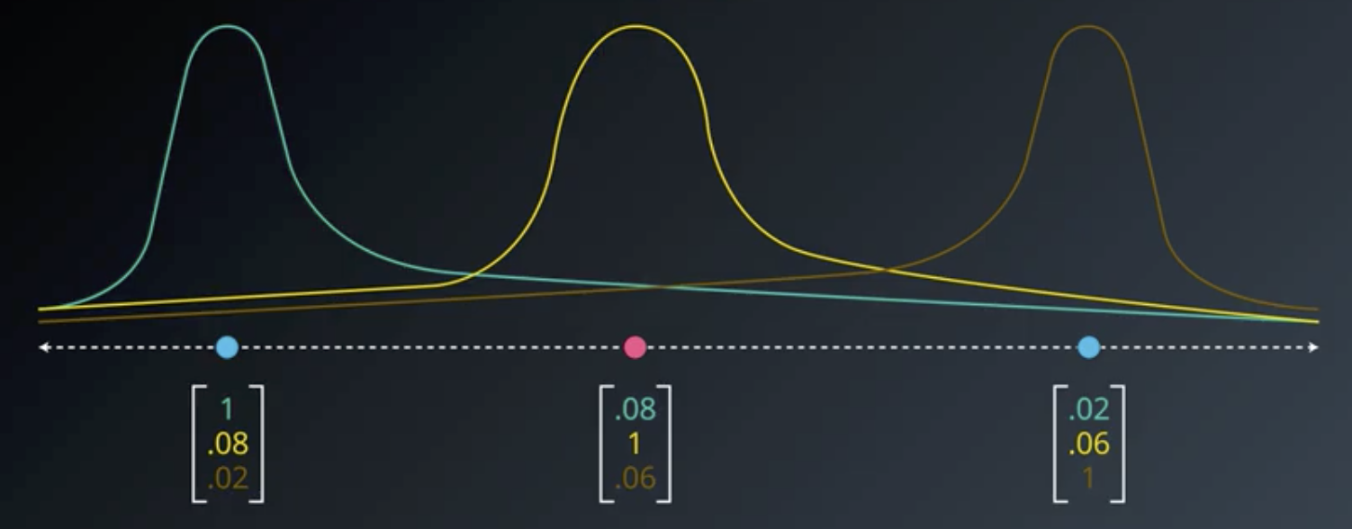
If we take the values of each of those functions and put them into a 3-dimensional vector space, then the red point would clearly be separable from the blue points by the plane shown below.
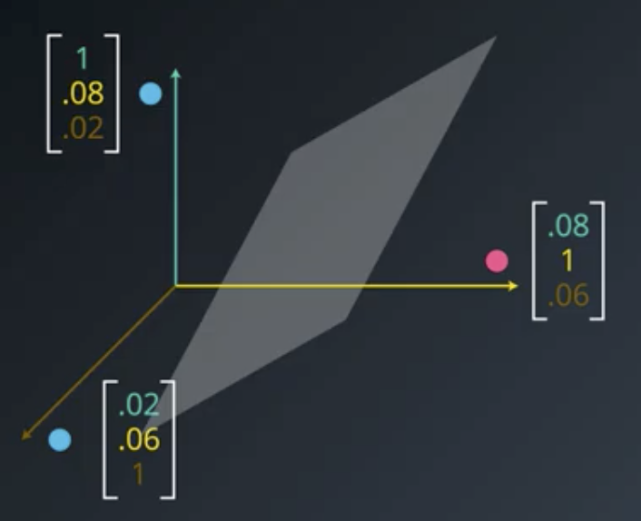
Suppose that the plane has an equation like the following:
$$2x-4y+z=-1$$

Those coefficients would be the values by which each of the constituent functions would be multiplied prior to summing them up. And, the equation for the line would be given by the constant term.

RBFs in Higher Dimensional Space
In a 3-dimensional space, the “mountain” is a gaussian paraboloid onto which the point is projected. The boundary is a plane which intersects the paraboloid, forming a circle which can be projected back down into the 2-dimensional space.

If there are multiple points, they are all treated similarly.

Wide versus Narrow RBFs
The $\gamma$ (“gamma”) parameter controls how wide or narrow the “mountains” are. A larger $\gamma$ means narrower peaks.

This has significant impacts in the algorithm. The classification boundaries on the left and right in the image below were created by large and small $\gamma$s, respectively.
Larger values of $\gamma$ will tend to overfit; smaller values will tend to underfit.