Linear Regression
Tricks
Linear regression involves moving a line such that it is the best approximation for a set of points. The absolute trick and square trick are techniques to move a line closer to a point.
Absolute Trick
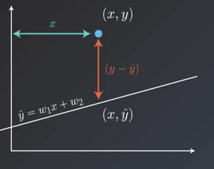
A line with slope $w_1$ and y-intercept $w_2$ would have equation $y = w_1x + w_2$. To move the line closer to the point $(p,q)$, the application of the absolute trick involves changing the equation of the line to
$$y = (w_1 + p\alpha)x + (w_2 + \alpha)$$
where $\alpha$ is the learning rate and is a small number whose sign depends on whether the point is above or below the line.
As an example, consider a line $y = -0.6x + 4$, a point $(x,y)=(-5,3)$, and $\alpha=0.1$. The point is below the line, so $\alpha$ is changed to be$\alpha=-0.1$. Following the application of the absolute trick, the equation of the line would be
$$y = (-0.6 + (-5)(-0.1))x + (4 - 0.1)$$
$$y = -0.1x + 3.9$$
Square Trick
A line with slope $w_1$ and y-intercept $w_2$ would have equation $y = w_1x + w_2$. The goal is to move the line closer to the point $(p,q)$. A point on the line with the same y-coordinate as $(p,q)$ might be given by $(p,q')$. The distance between $(p,q)$ and $(p,q')$ is given by $(q-q')$. Following application of the square trick, the new equation would be given by
$$y = (w_1 + p(q-q')\alpha)x + (w_2 + (q-q')\alpha)$$
where $\alpha$ is the learning rate and is a small number whose sign does not depend on whether the point is above or below the line. This is due to the inclusion of the $(q-q')$ term that takes care of this implicitly.
As an example, consider a line $y = -0.6x + 4$, a point $(x,y)=(-5,3)$, and $\alpha=0.01$.
$$q' = -0.6(-5) + 4 = 3 + 4 = 7$$ $$(q - q') = (3 - 7) = -4$$
Then, the new equation for the line would be given by
$$y = (-0.6 + (-5)(-4)(0.01))x + (4 + (-4)(0.01))$$ $$y = -0.4x + 3.96$$
Gradient Descent
The more formal way by which regression works is called gradient descent. For a given line and set of points, we can define a function that calculates an “error.” This error gives us some sense of how far the line is from the points. After moving the line, this error would be recalculated and should decrease. Gradient descent involves determining which direction to move the line that would decrease the error the most.
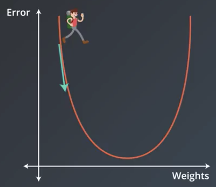
More technically, it involves taking the derivative, or gradient, of the error function with respect to the weights, and taking a step in the direction of largest decrease.
$$w_i \rightarrow w_i - \alpha \frac{\partial}{\partial w_i}Error$$
Following several similar steps, the function will arrive at either a minimum or a value where the error is small. This is also referred to as “decreasing the error function by walking along the negative of its gradient.”
Mean Absolute Error
The two most common error functions for linear regression are the mean absolute error and the mean squared error. Consider a point $(x,y)$ and a line $(x,\hat{y})$. The vertical distance from the point to the line is given by $y-\hat{y}$.
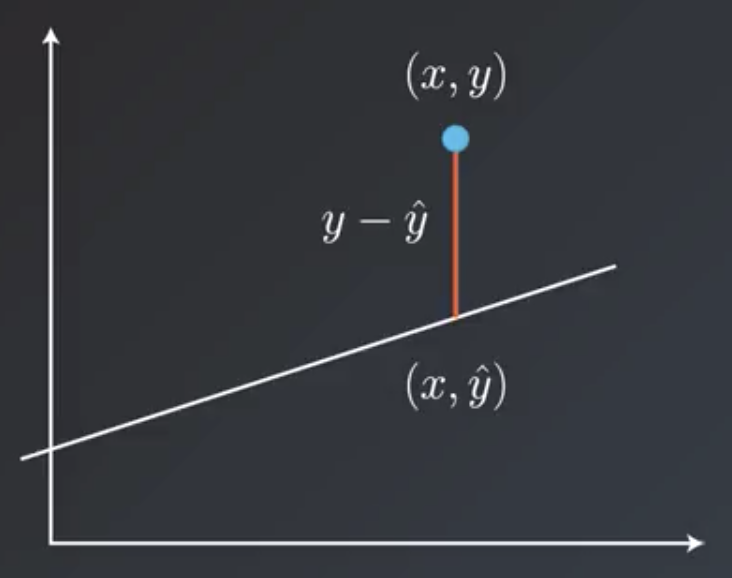
Then, the total error is the sum of all these distances from the points to the line in the dataset divided by the number of points, $m$.
$$Error = \frac{1}{m} \sum^m_{i=1}|y-\hat{y}|$$
For example, consider the line $y = 1.2x + 2$ and the points $(2, -2), (5, 6), (-4, -4), (-7, 1), (8, 14)$:
| # | Point | $\hat{y}$ | $|y - \hat{y}|$ |
|---|---|---|---|
| 1 | (2, -2) | 2.4 | 6.4 |
| 2 | (5, 6) | 6 | 2 |
| 3 | (-4, -4) | -4.8 | 1.2 |
| 4 | (-7, 1) | -8.4 | 7.4 |
| 5 | (8, 14) | 9.6 | 2.4 |
$$Error = \frac{1}{5} (6.4 + 2 + 1.2 + 7.4 + 2.4) = 3.88$$
Mean Squared Error
The mean squared error is similar to the mean absolute error. The extra factor of $\frac{1}{2}$ is for convenience later.
$$Error = \frac{1}{2m} \sum^m_{i=1}(y-\hat{y})^2$$
| # | Point | $\hat{y}$ | ($y - \hat{y})^2$ |
|---|---|---|---|
| 1 | (2, -2) | 2.4 | 40.96 |
| 2 | (5, 6) | 6 | 4 |
| 3 | (-4, -4) | -4.8 | 1.44 |
| 4 | (-7, 1) | -8.4 | 54.76 |
| 5 | (8, 14) | 9.6 | 5.76 |
$$Error = \frac{1}{(2)(5)} (40.96 + 4 + 1.44 + 54.76 + 5.76) = 10.692$$
Derivative of the Error Function
The absolute trick and square trick and the mean absolute error and mean squared error are actually the same thing.
By using the square trick, we actually are taking a gradient descent step:
$$Error = \frac{1}{2}(y-\hat{y})^2$$
$$\frac{\partial}{\partial w_1} Error = \frac{\partial Error}{\partial \hat{y}} \frac{\partial \hat{y}}{\partial w_1} = -(y-\hat{y})x$$
$$\frac{\partial}{\partial w_2} Error = \frac{\partial Error}{\partial \hat{y}} \frac{\partial \hat{y}}{\partial w_2} = -(y-\hat{y})$$
Gradient step:
$$w_i \rightarrow w_i - \alpha \frac{\partial}{\partial w_i} Error$$
By using the absolute trick, we actually are taking a gradient descent step as well.
$$Error = |y - \hat{y}|$$
$$\frac{\partial}{\partial w_1} Error = \pm x$$
$$\frac{\partial}{\partial w_2} Error = \pm 1$$
The $\pm$ is based on whether the point is above or below the line.
Gradient step:
$$w_i \rightarrow w_i - \alpha \frac{\partial}{\partial w_i} Error$$
Mean versus Total Squared (or absolute) Error
The total squared error, $M$, is the sum of errors at each point.
$$M = \sum^m_{i=1} \frac{1}{2} (y - \hat{y})^2$$
The mean squared error, $T$ is the average of these errors.
$$T = \sum^m_{i=1} \frac{1}{2m} (y - \hat{y})^2$$
So, the total squared error is just a multiple of the mean squared error, because $M = mT$. When using regression in practice, algorithms help determine a good learning rate to work with. Whether the mean error or the total error is selected, it ultimately will just amount to picking a different learning rate, and the algorithms will just adjust accordingly. So, either mean or total squared error can be used.
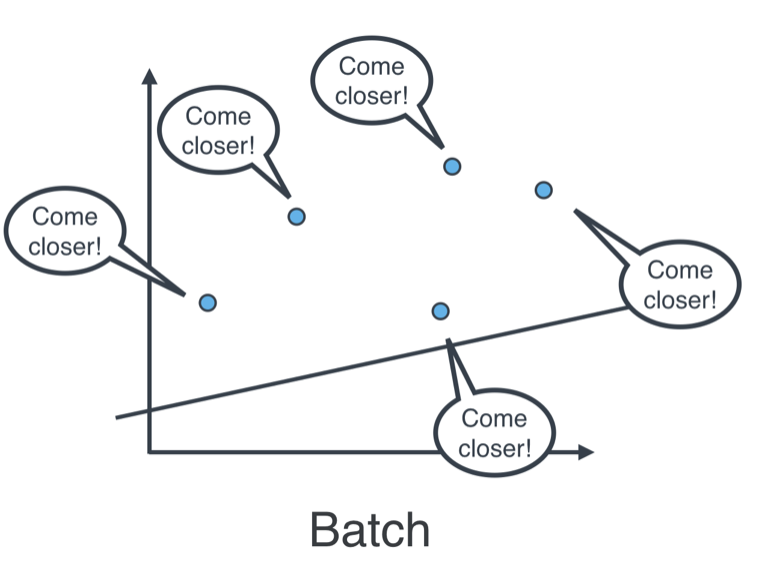
Batch versus Stochastic versus Mini-Batch Gradient Descent
- Batch gradient descent: applying on of the tricks at every point in the data, all at the same time.
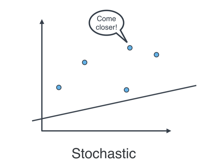
- Stochastic gradient descent: applying one of the tricks at every point in the data, one by one.
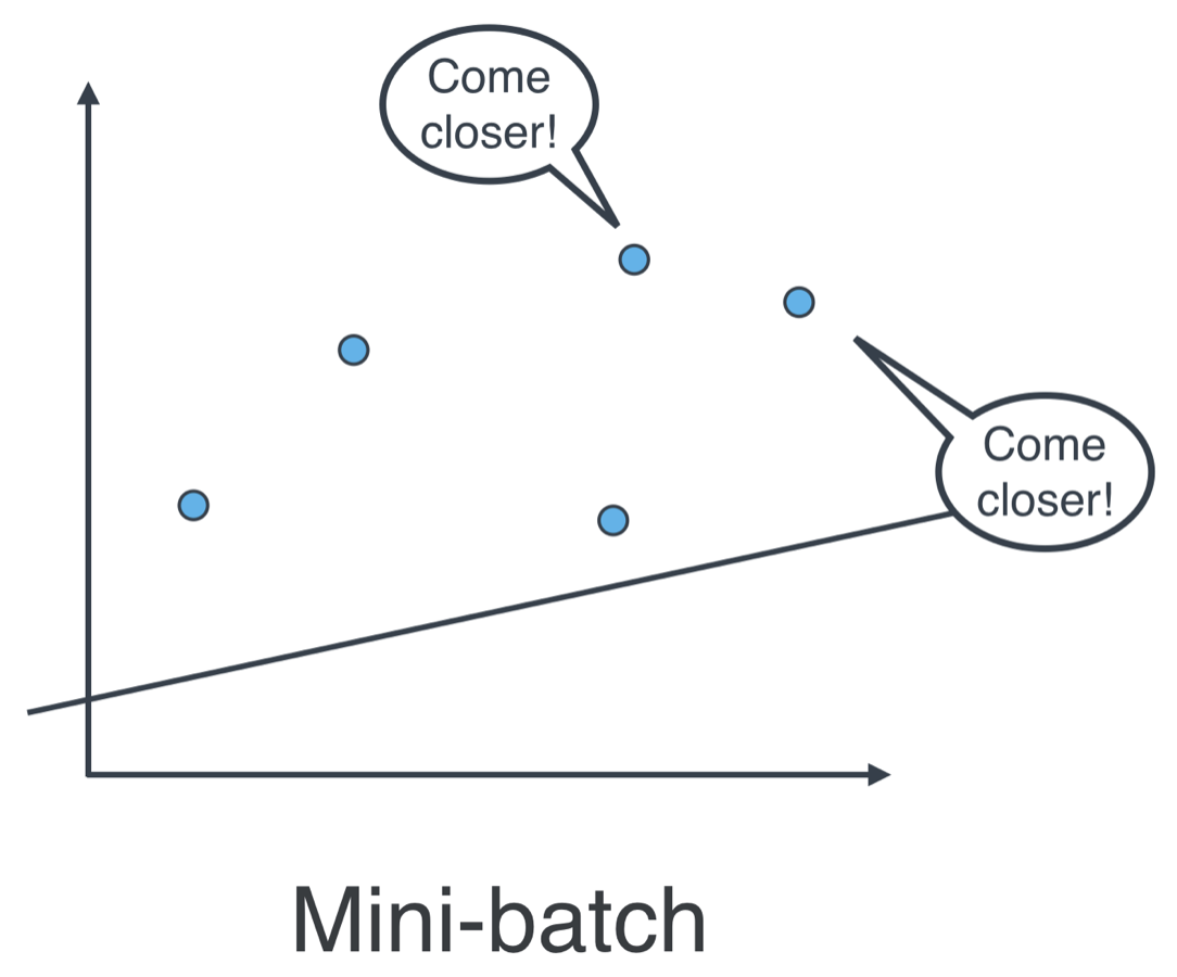
- Mini-batch gradient descent: applying one of the tricks to a small batch of points, with each small batch containing roughly the same number of points. Computationally, this is the most efficient approach, and the one that is used in practice.
Mean Squared versus Mean Absolute Errors
One difference between these two error formulations is that the mean squared error is a quadratic function, whereas mean absolute error is not. What this means practically is that in some point distributions the mean squared error will give better results.
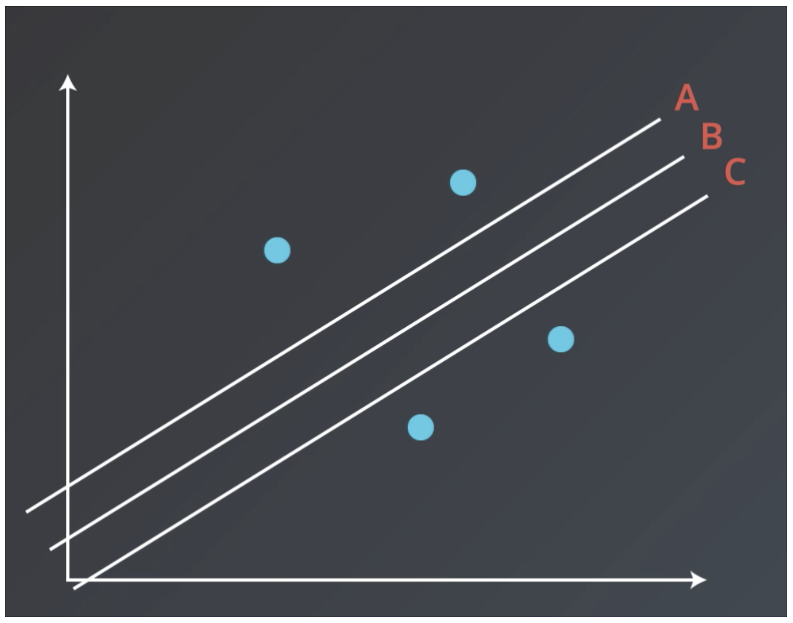
Lines A, B, and C have the same mean absolute error on the points distributions shown, but B has the smallest mean squared error.
Generalizing to Higher Dimensions
Previous examples have been two-dimensional problems. For example, a model might take as an input house size and output house price. In 2-dimensional models, the prediction is a line.
$$Price = w_1(size) + w_2$$
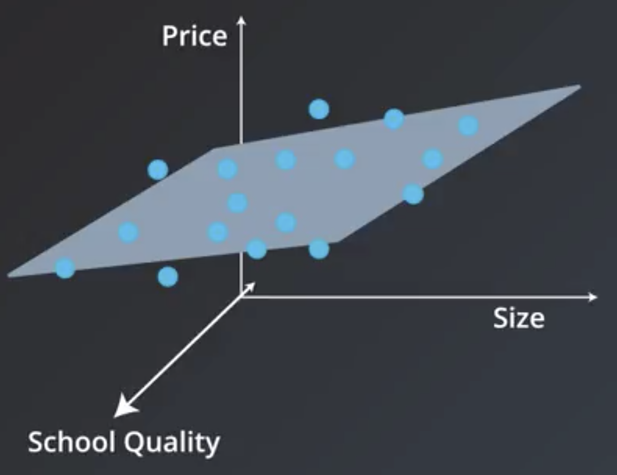
Consider a situation where house size and nearby school quality are both factors used by a model that predicts house price. In this situation, the graph becomes 2-dimensional, and the prediction becomes a plane.
$$Price = w_1(school\ quality) + w_2(size) + w_3$$
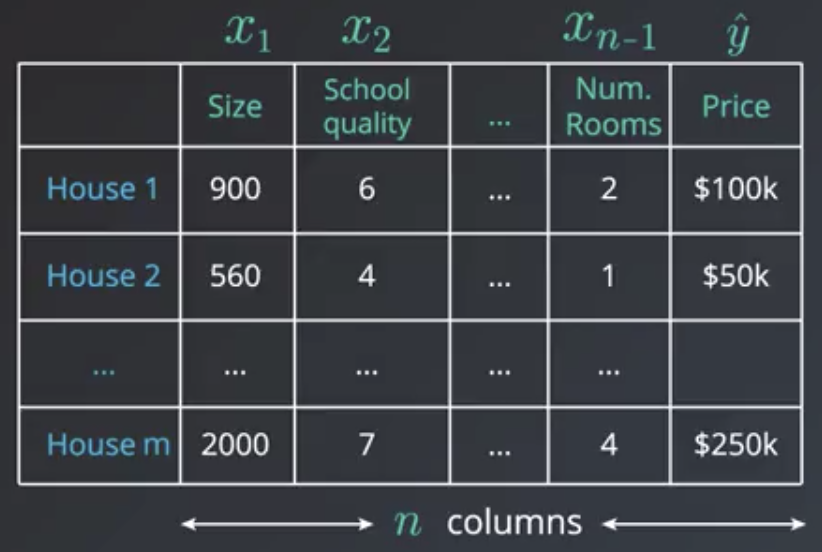
In the more general $n$-dimensional case there are $n-1$ input features ($x_1, x_2, …, x_{n-1}$, also known as predictors or independent variables) and $1$ output feature ($\hat{y}$, also known as dependent variables). The prediction becomes an $n-1$ dimensional hyperplane.
$$\hat{y} = w_1 x_1 + w_2 x_2 + … + w_{n-1} x_{n-1} + w_n$$
The algorithm in this more general situation is exactly the same as the 2-dimensional case.
The instructor notes that there is actually a closed form solution to finding the set of coefficients, $w_1, … w_{n-1}$, that give the minimum mean squared error. Using this closed form solution requires solving a system of $n$ equations and $n$ unknowns, however, which, depending on the dataset, may be computationally expensive to the point of being impractical. So, in practice, gradient descent is almost always used. It does not give an exact answer in the same way that a closed-form solution would, but the approximate solution it does provide is almost always adequate.
Linear Regression Warnings
Linear regression comes with a set of implicit assumptions and is not the best model for every situation.
Linear Regression Works Best when the Data is Linear
If the relationship is not linear, then you can:
- Make adjustments (transform the data),
- Add features, or
- Use another kind of model.
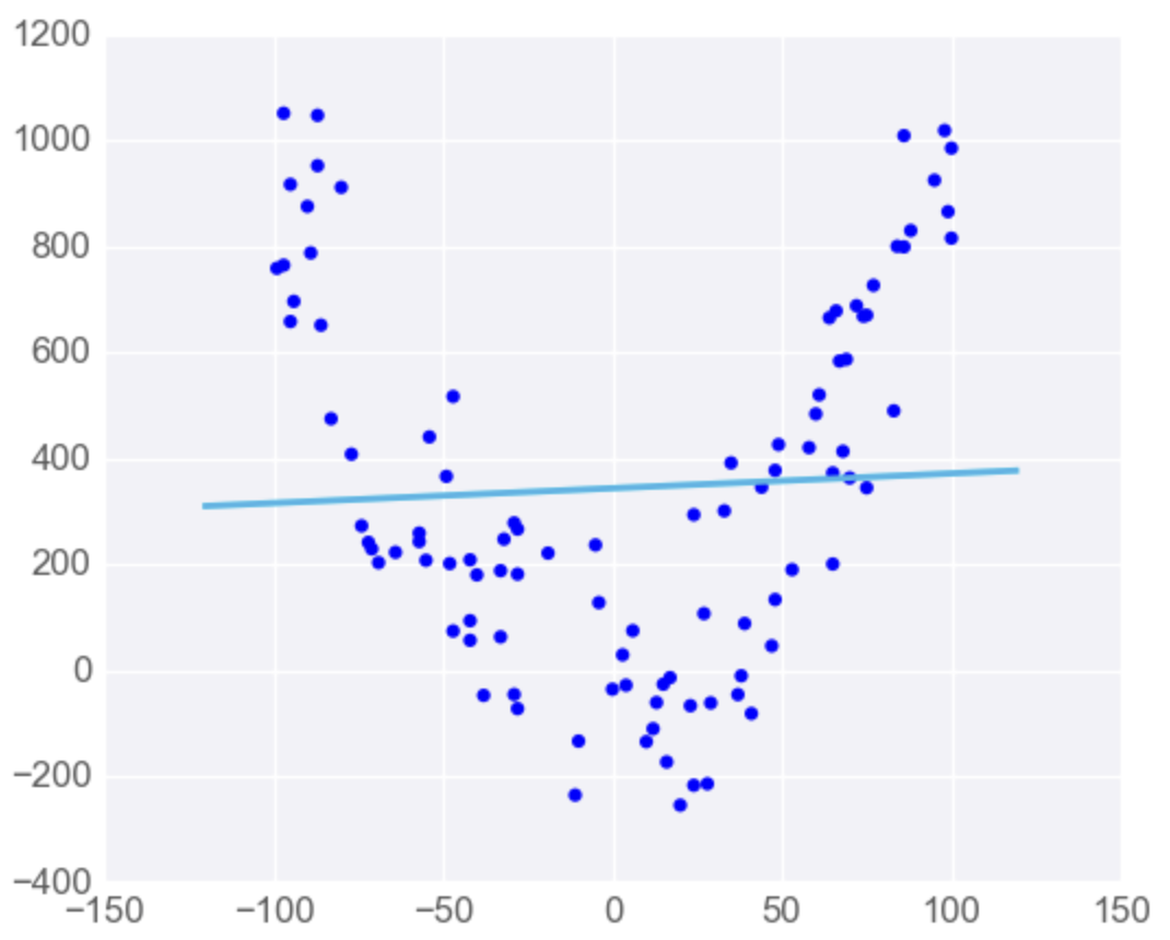
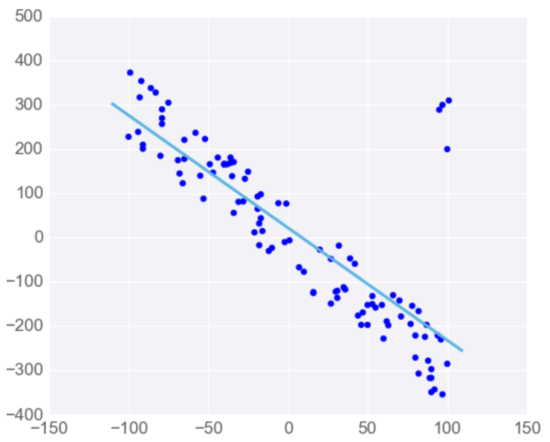
Linear Regression is Sensitive to Outliers
If the dataset has some outlying extreme values that don’t fit a general pattern, they can have a very large effect.
Polynomial Regression
Some datasets are clearly not suited to linear regression. a polynomial may work better.
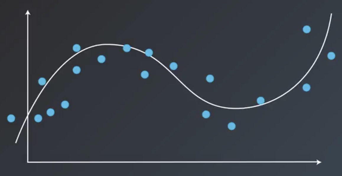
In these situations, instead of a line, a polynomial like the following could be used instead.
$$\hat{y} = w_1 x^3 + w_2 x^2 + w_3 x + w_4$$
The algorithm to solve this equation is the exact same thing. We take the mean absolute or mean squared error and take the derivative with the four variables. Then, we use gradient descent to modify these four weights and minimize the error. This algorithm is known as polynomial regression.
Regularization
Regularization is a concept that works for both classification and regression. It is a technique to improve our models and make sure they don’t overfit.
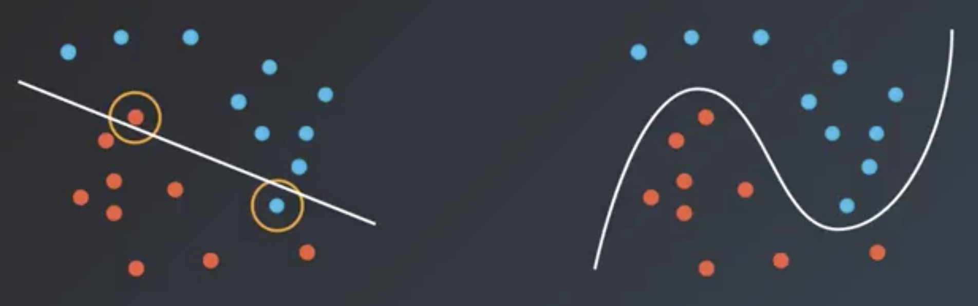
In machine learning, there is often a tradeoff between accuracy and generalizability. In the image below, the linear model is not as accurate as the polynomial. Specifically, the linear model makes two misclassifications. But, the linear model is simpler and may generalize better to other datasets better than the polynomial model, which is more complex and accurate but may be overfit to this particular dataset.
Regularization is a way to take the complexity of the model into account when calculating the overall error of the model. So, the overall error of a given model is redefined as any misclassifications plus the complexity of the model.
L1 Regularization
In L1 Regularization, the absolute value of the coefficients is added to the error.
For example, in the case of the following polynomial model:
$$2 x_1^3 - 2 x_1^2 x_2 - 4 x_2^3 + 3 x_1^2 + 6 x_1 x_2 + 4 x_2^2 + 5 = 0$$
$$Error = |2| + |-2| + |-4| + |3| + |6| + |4| = 21$$
In the case of the following linear model:
$$3 x_1 - 4 x_2 + 5 = 0$$
$$Error = |3| + |4| = 7$$
L2 Regularization
L2 Regularization is similar, except it involves adding the squares of the coefficients.
For the same polynomial above:
$$Error = 2^2 + (-2)^2 + (-4)^2 + 3^2 + 6^2 + 4^2 = 85$$
For the same linear model above:
$$Error = 3^2 + 4^2 = 25$$
Regularization Tradeoffs
The type of regularization to use depends on the model’s use-case. If the model will be used in medical or aerospace applications, maybe low error is required and high complexity is okay. If the model is used to recommend videos or friends on a social networking site, maybe scalability and therefore simplicity and speed need to be prioritized.
The amount of regularization applied to an algorithm is determined by a parameter called lambda ($\lambda$), which is a scalar by which the regularization term is multiplied.
| L1 Regularization | L2 Regularization |
|---|---|
| Computationally Inefficient (unless data is sparse) | Computationally Efficient |
| Sparse Outputs | Non-Sparse Outputs |
| Feature Selection (may set some features to 0) | No Feature Selection |
Feature Scaling
Feature scaling is a way of transforming data into a common range of values. There are two common scalings: standardizing and normalizing.
Standardizing
Standardizing is the most common technique for feature scaling. Data is standardized by subtracting the mean of each column from each value, then dividing it by the standard deviation of the column.
df["height_standard"] = (df["height"] - df["height"].mean()) / df["height"].std()
Normalizing
Normalizing is performed by scaling data to a value between 0 and 1.
df["height_normal"] = (df["height"] - df["height"].min()) / (df["height"].max() - df['height'].min())
When Should Feature Scaling be Used?
- When the algorithm uses a distance-based metric to predict
- For example, Support Vector Machines and K-Nearest Neighbors (K-NN) both require that the input data be scaled.
- When using regularization
- For example, when one feature is on a small range (0-10) and another is on a large range (0-1000), regularization will unduly punish the feature with the small range.
- Note that feature scaling can also speed up convergence of machine learning algorithms, which may be an important consideration.