Training Considerations
In practice, when training neural networks, there are many ways the process can go wrong. For example:
- the architecture can be poorly chosen,
- the data can be noisy, and
- the training can take far too long.
The purpose of these notes is to capture several ways to optimize training of neural networks.
Simplicity
One simple rule of thumb in machine learning: whenever we can choose between a simple model that works and a complicated model that may perform slightly better, we always go for the simpler model.
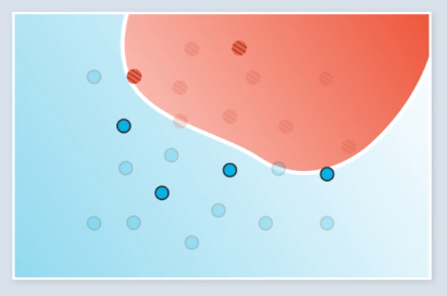
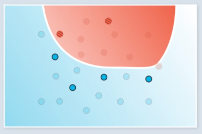
For example, a simple and complex model is shown on the left and right, respectively, of the image below. It appears the complex model outperforms on the training data, which is shown in the image.
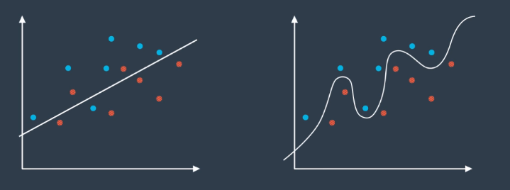
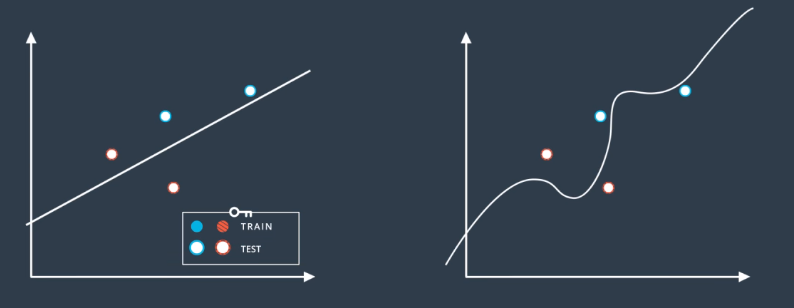
Once the test data is introduced, it is clear the simple model actually performs better. This is a simple example, but the principle generalizes to all machine learning.
Types of Model Error
There are two main types of model error in machine learning:
- Overfitting: model is too complex for the data. This is an error due to variance.
- Underfitting: model is too simple for the data. This is an error due to bias.
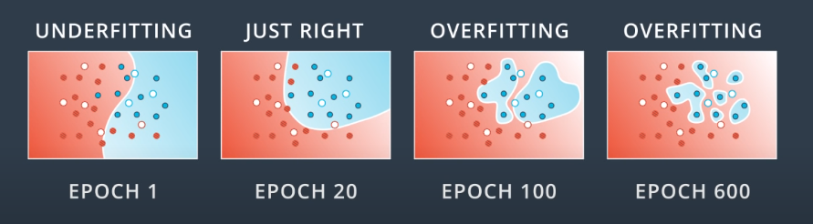
This is shown graphically in the following image. Examples of network architectures are shown at the top.
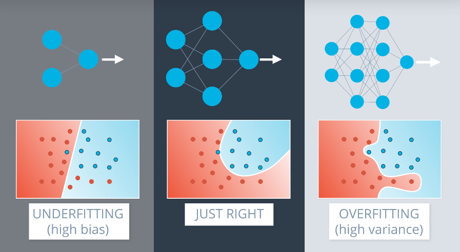
Unfortunately, it is very hard to find the right architecture for a neural network. The best approach is to err on the side of a slightly overly-complex model, and then apply certain techniques to prevent overfitting on it.
Early Stopping
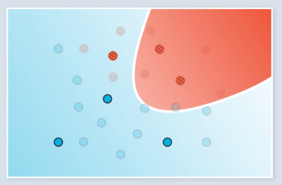
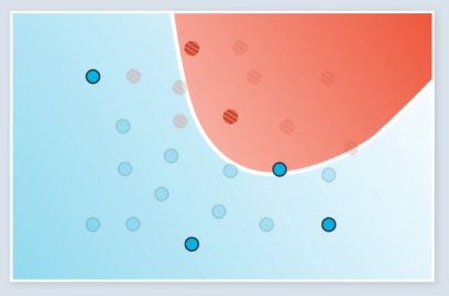
Early stopping is a technique that prevents models from overfitting the training data. It involves stopping training once a point in the training is reached where the testing error begins to increase and diverge from the training error.
Assume that we are following the recommendation from the previous section, and we have a model that is slightly more complex than particular data problem requires. As we train the model, we can expect the model boundaries to change as follows.
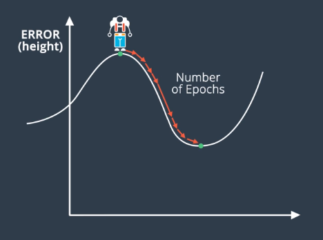
The following image introduces model complexity graphs, which are graphs that show the training and testing errors as a function of the training epoch.
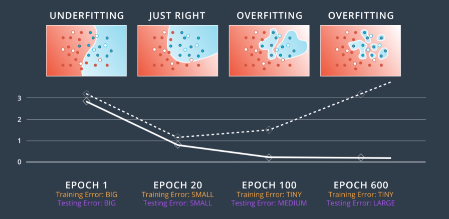
In general, the training curve decreases since as we train the model, we fit the training data better and better. The testing error is large when we’re under-fitting and decreases as the model generalizes better and better. Eventually, it increases and diverges from the training error as the model begins to overfit.
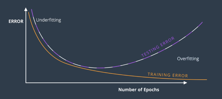
In summary, the early stopping technique is to perform gradient descent until the testing error stops decreasing and starts to increase. At that point, we stop.
Regularization
Regularization is a means of penalizing large weights in the model.
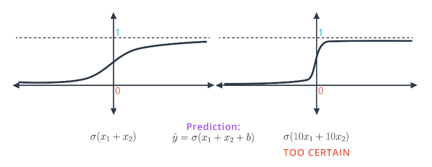
Consider a situation where we are attempting to split two points, and have two possible models that could be used. We are trying to find the model with the smallest error. Recall that the predictions are given by $\hat{y} = \sigma(w_1 x_1 + w_2 x_2 + b)$.
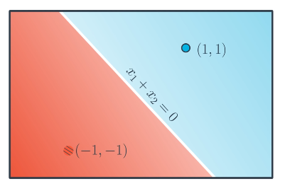
- Solution 1: $x_1 + x_2$
- $\sigma(1+1)=0.88$
- $\sigma(-1-1)=0.12$
- Solution 2: $10 x_1 + 10 x_2$
- $\sigma(10+10)=0.9999999979$
- $\sigma(-10-10)=0.0000000021$
The second solution clearly would give a smaller error. But, the model is overfit in a subtle way. The sigmoid functions for the two models are shown below, and as shown, the second solution is too certain and its sigmoid function is too steep. As a result, it is much harder to do gradient descent since the deriviatives are mostly close to 0, except where it crosses the y-axis and becomes very large. It is difficult to train under these circumstances.
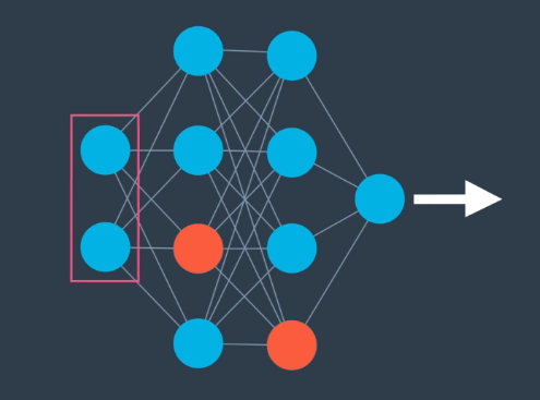
Since overfit models are more certain, this can be a difficult type of error to prevent. This is where regularization comes in and enables us to penalize large weights. The regularization terms are highlighted in the image below.
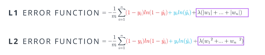
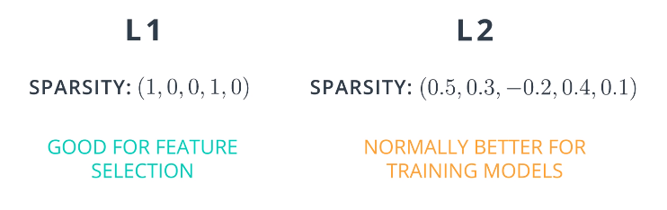
There are two types of regularization: L1 and L2. Which to use depends on our goals and application. L1: tends to result in sparse vectors. L2: tries to maintain all weights homogeneously small.
Dropout
Dropout is a means of preventing some parts of a neural network from “overpowering” the entire network by having relatively large weights.
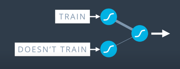
The impact of this imbalance is that some of the nodes become much more influential than others. To combat this, as we progress through the training epochs, we turn off certain nodes so that the other nodes have to “pick up the slack” and take more part in the feedforward and backpropagation.
Practically, this is implemented by passing a parameter to the algorithm that is the probability that each node will be dropped in a given epoch. For example, passing 0.2 as that parameter would mean a 20% chance each node is dropped. This technique is very common.
Random Restart
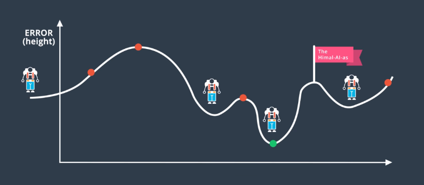
Random Restart is a means of solving the local minima problem. Local minima is a phenomenon where the network weights settle into a configuration where gradient descent has “gotten stuck” where the error is relatively, but not globally, low.
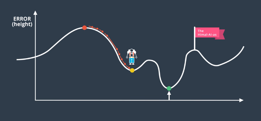
Using the mountain analogy discussed elsewhere, random restart involves starting training from random points on the overall gradient, and then performing gradient descent.
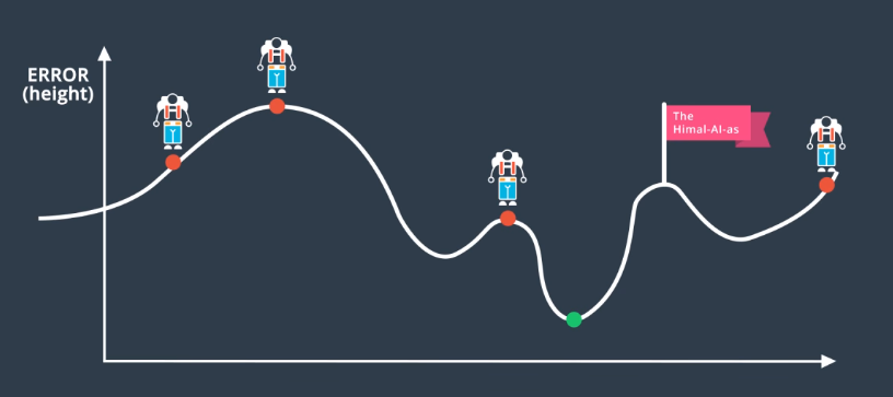
This makes it more likely that the global minimum (or, at least, a better local minimum) will be found.
Vanishing Gradient Problem
The Vanishing Gradient problem is especially relevant when using the sigmoid activation function. The problem is that the gradient is very flat (derivative close to 0) at locations far from the y-axis.
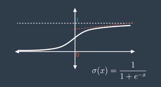
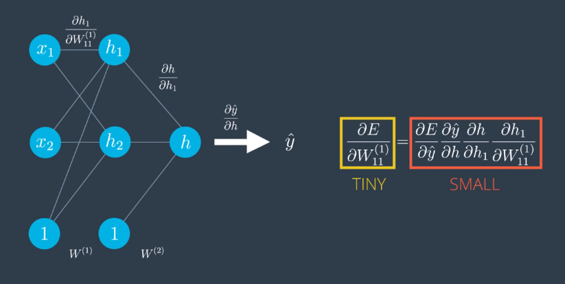
Recall the derivative of the error function with respect to a weight is the product of all the derivatives calculated at the nodes in the corresponding path to the output. All those derivatives may be small because the sigmoid activation function is being used. As a result, their product may be tiny.
This means that gradient descent may operate very slowly.
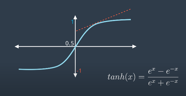
Other Activation Functions
The best way to address the vanishing gradient problem is to use other activation functions.
One is the Hyperbolic Tangent Function. The function is shaped similarly to sigmoid, but, since the range is from $-1$ to $1$ the derivative is larger. This seemingly minor change actually led to many advances in neural networks.
Another is the Rectified Linear Unit (ReLU). This is a very simple function that uses the larger value of $x$ and $0$. This function is commonly used instead of sigmoid. It can improve training significantly without sacrificing much accuracy. Note that if $x$ is positive the deriviative is $1$.
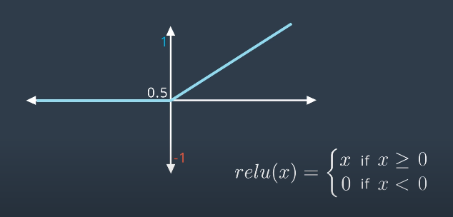
Note that in both plots above, the origin should be labeled with a value $y=0$, not $y=0.5$.
The following image shows a simple neural network that uses ReLU for the hidden layers and sigmoid for the output, since the final output still needs to be a probability between $0$ and $1$.
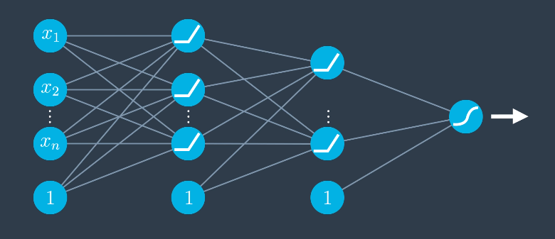
If the final unit is left as a ReLU, we can end up with regression models that predict a value. This is important for recurrent neural networks.
Batch versus Stochastic Gradient Descent
Batch gradient descent is the methodology we have been employing so far. Training a neural network involves taking a number of steps down a gradient, where each step is called an “epoch.”
In batch gradient descent, all of the data is run through the neural network and the associated error is backpropagated through the network. This works and does improve the model, but we generally have many data points, so these training steps end up being huge matrix computations that use a lot of memory. Since this must be done for every single step, the computation and time cost can become significant.
If the data is well-distributed, a small subset of the data may give us a pretty good idea of what the gradient would be. This is what stochastic gradient descent comes in.
Stochastic gradient descent involves running gradient descent on small subsets of the available data during each step. In the following example, we have 24 total points, and each training epoch is run on a random batch of 6 of them. The first 2 of four total training steps are shown.
Previously, each training step would be run once on all of the data. With stochastic gradient descent, training on all the data required 4 steps. The steps we took were less accurate, but in practice, it is better to take several slightly inaccurate steps than one good one.
Learning Rate
Selecting an appropriate learning rate is complex. In general, large learning rates mean you are taking huge steps and it will probably work well initially. But, it may not reach the actual local minimum. It is likely to make the training process chaotic. In general, if training the model is not working, try decreasing the learning rate.
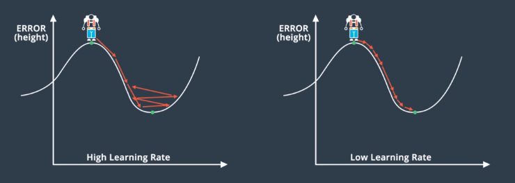
It is also possible to use learning rates that change as a function of the gradient step. The best learning rates are those that decrease as the model is getting closer to a solution. The rules are:
- If the gradient is steep, take long steps.
- If it gradient is flat, take small steps.
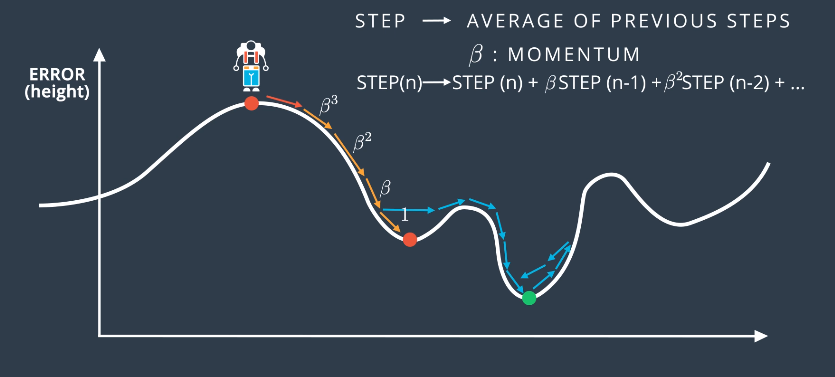
Momentum
Another way to solve the local minimum problem is to introduce a momentum to the gradient descent. In the analogy, this would mean walking quickly and with momentum to “power through” small increases in the error function, so that a lower minimum can be found.
Practically, this often means taking steps that are a weighted average of the past few steps. Momentum is a constant $\beta$ that attaches to the steps as follows:
$$STEP(n) \rightarrow STEP(n) + \beta STEP(n-1) + \beta^2 STEP(n-2) + …$$
In this way, the steps that happened several back will matter less than the more recent ones. Algorithms that use momentum terms work very well, in practice.