Neural Network Architecture
This is a continuation of the notes on Neural Networks.
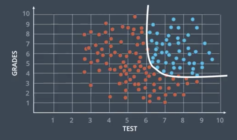
Neural networks are capable of coping with data that is not linearly separable. The probability function and optimization process are similar to that for linearly separable data.
Neural Network Architecture
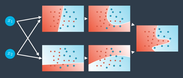
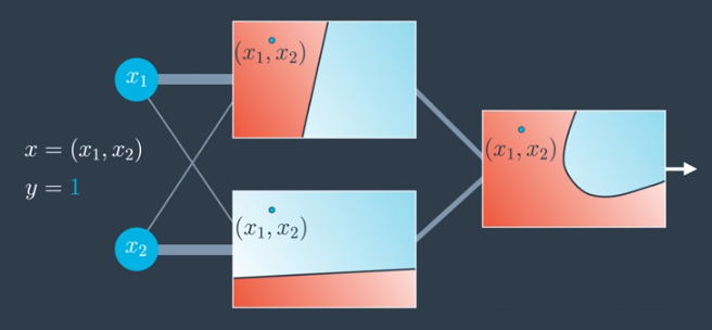
Training a model to correctly classify non-linear data like that shown above requires superimposing multiple neural networks on top of one another.
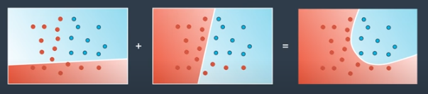
Practically, this means checking the probability in both of these neural networks individually and then combining the result to get the probability in the resulting probability space.
- Determine probabilities for each network individually,
- Add these results together,
- Apply the Sigmoid function to the combined result.
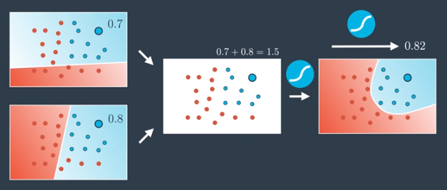
This calculation is run for every point in the plane.
Weighting the Component Networks
It is also possible to weight the input neural networks. For example, the model on the top left of the image below could be weighted more strongly than the model on the bottom left.
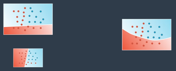
For example, the output of the top neural network could be given a weight of 7. The bottom could be given a weight of 5. An arbitrary bias of 6 could also be assigned.
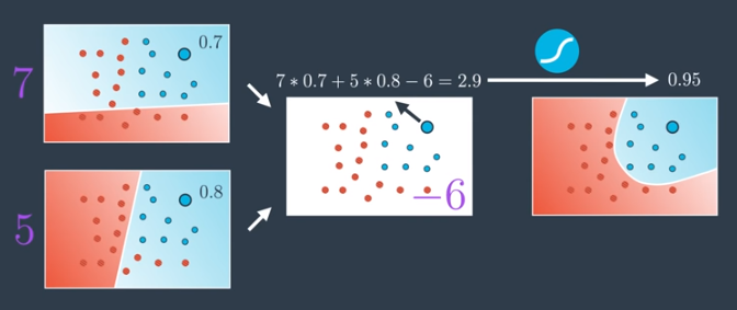
Note that this exactly how neural networks themselves operate, except instead of inputs to a neural network we have neural networks, themselves.
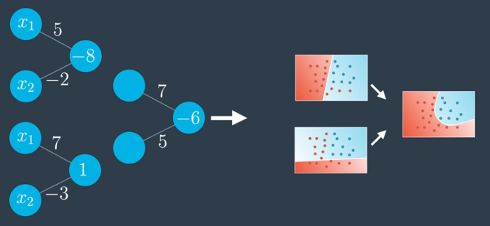
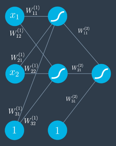
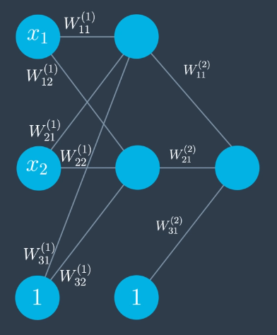
By cleaning up and consolidating the network above, we arrive at the following.
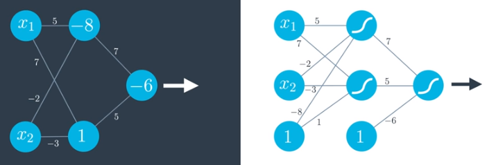
Note that the following two networks are actually identical. One uses a notation where the bias (-6) is placed inside the node. The other uses a notation where the bias comes from a single node with constant input 1 where the edges are weighted by the bias. In both cases, the sigmoid activation function is used.
Multiple Layers
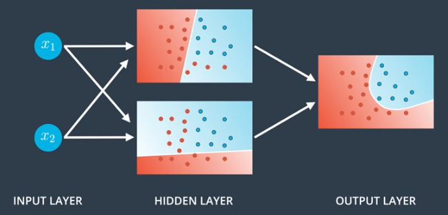
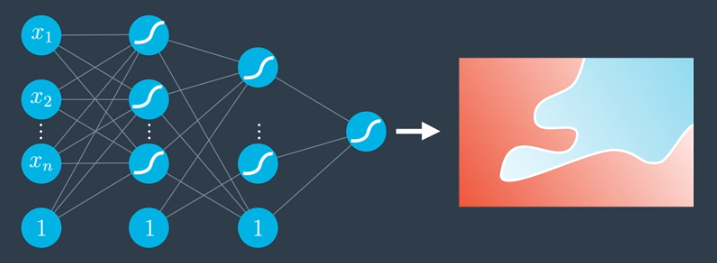
In general, neural networks have at least 3 layers:
- Input Layer: contains the inputs to the model.
- Hidden Layer: the set of linear models created using the inputs.
- Output Layer: where the hidden layers are combined to obtain a nonlinear model.
Neural networks can be much more complex than the examples shown above. In particular, we can:
- Add more nodes to the input, hidden, and output layers, and
- Add more layers.
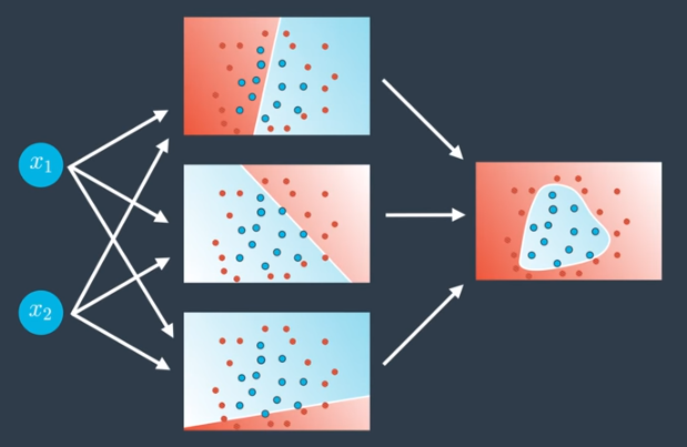
Adding More Nodes
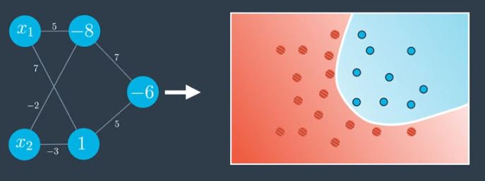
Adding more nodes to the hidden layer enables creation of more complex outputs, such as the triangular region shown below.
Adding more nodes to the input layer means the data space is higher dimensional. For example, in the network architecture below, the space is three-dimensional, the linear models in the hidden layers are planes, and the output layer bounds a nonlinear region in three space.
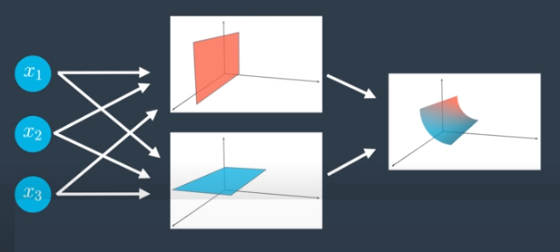
In general, if we have n dimensions in the input layer, we are living in n space.
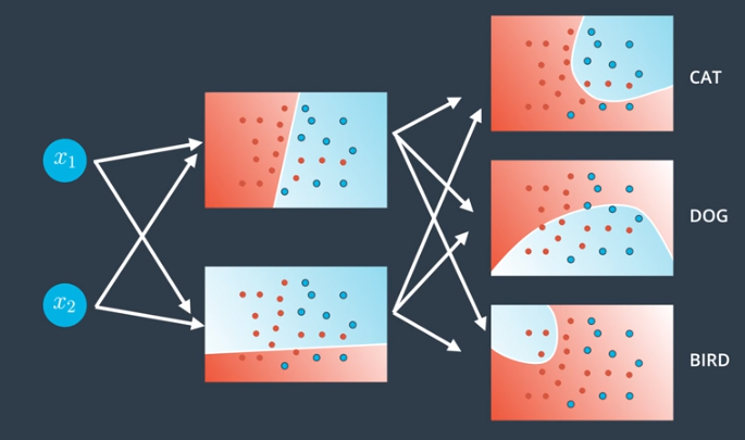
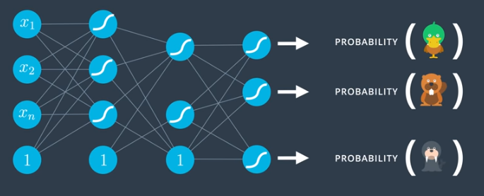
Adding more dimensions to the output layer means we have more outputs, and we are performing more complex, multiple-class classification.
Adding More Layers
If we add more layers, we have a deep neural network. Our nonlinear models combine to create even more nonlinear models.
This can be done many times, creating highly complex nonlinear models. Many of the models in real life, specifically, in applications such as self-driving cars and game-playing agents, have many hidden layers.
Multi-class Classification
When using neural networks to perform multi-class classification, the number of outputs must match the number of classifications. Then, we use the softmax function on those outputs to obtain well-defined probabilities.
Feedforward
Feedforward is the process neural networks use to turn an input into an output.
Feedforward in Perceptrons
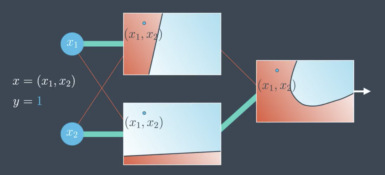
Consider the example shown in the image below. The input is given by $x=(x_1,x_2)$, and the label is $y=1$.
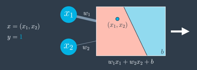
The perceptron receives the data point, $(x_1,x_2)$. The perceptron plots the point and outputs the probability that thte point is blue. Here, since the point is in the red area, the output would be a small number since the point is not very likely to be blue. But, in this case the point is blue, so the model does not appear to be very good.
Feedforward in Neural Networks
Feedforward operates in a similar manner for neural networks.
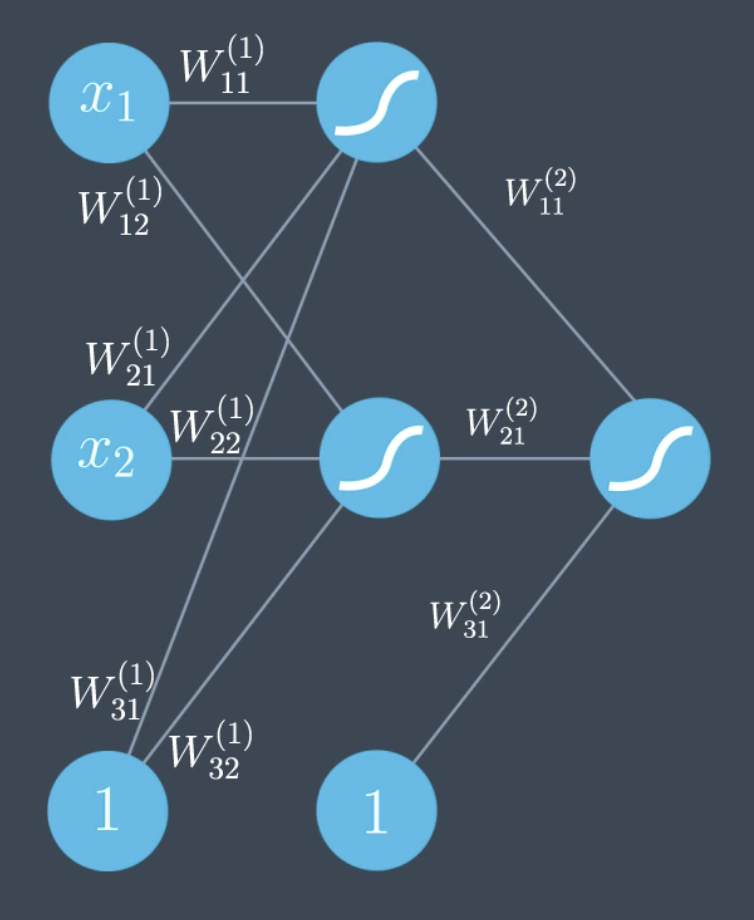
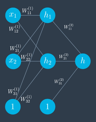
To discuss more specifically, introduce the following notation:
- $W^{(2)}$ - indicates the weight belongs to the second layer.
- $W_{12}$ - indicates the weight is between the first node in the layer that is the input to the edge, and the second node in that layer that is the output to the edge.
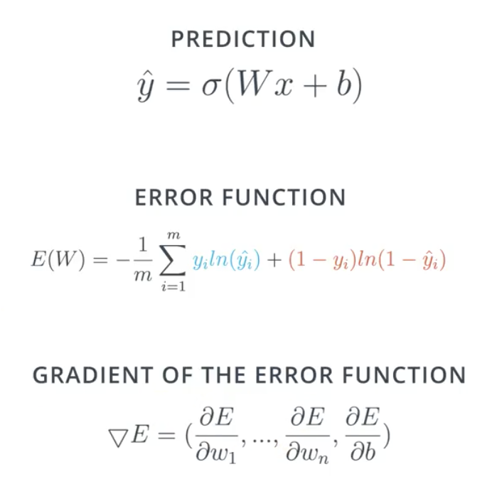
The output prediction, $\hat{y}$, is given by
$$\hat{y} = \sigma \Bigg( \begin{matrix}W_{11}^{(2)} \\ W_{21}^{(2)} \\ W_{31}^{(2)} \end{matrix} \Bigg) \sigma \Bigg( \begin{matrix}W_{11}^{(1)} & W_{12}^{(1)} \\ W_{21}^{(1)} & W_{22}^{(1)} \\ W_{31}^{(1)} & W_{32}^{(1)} \end{matrix} \Bigg) \Bigg( \begin{matrix}x_1 \\ x_2 \\ 1 \end{matrix} \Bigg)$$
A more compact representation of the same equation is shown below.
$$\hat{y} = \sigma \circ W^{(2)} \circ \sigma \circ W^{(1)}(x)$$
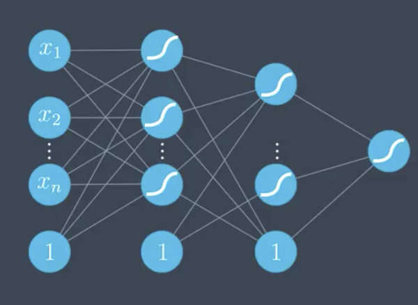
For a 3-layer neural network, like that shown below, the equation that follows would be used.
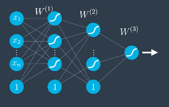
$$\hat{y} = \sigma \circ W^{(3)} \sigma \circ W^{(2)} \circ \sigma \circ W^{(1)}(x)$$
Error Function
The error function for neural networks is the same as before. The only difference is that the formula for the prediction, $\hat{y}$, is more complicated.
$$E(W) = -\frac{1}{m} \sum_{i=1}^m y_iln(\hat{y_i}) + (1-y_i) ln(1-\hat{y}_i)$$
Backpropagation
Backpropagation is how neural networks are trained. It consists of the following sequence of steps:
- Doing a feedforward operation.
- Comparing the output of the model with the desired output.
- Calculating the error.
- Running the feedforward operation backwards (backpropagation) to spread the error to each of the weights.
- Use this to update the weights and get a better model.
- Repeat steps 1 through 5 until the model is good.
High-Level Example
Consider the example in the following image. The point is misclassified by one of the neural networks, and correctly classified in the other.
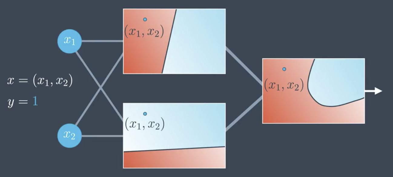
Since the model incorrectly classifies the point, the impact of backpropagation will be to:
- Increase the weight of the neural network that correctly classifies the point and decrease the weight of the neural network that incorrectly classifies the point,
- Change the weights of each of the two linear models in the hidden layer in order to better classify the point.
Note that in the image above the bias is not shown, for clarity, but in reality the bias would change as well.
Backpropagation Math
Perceptron
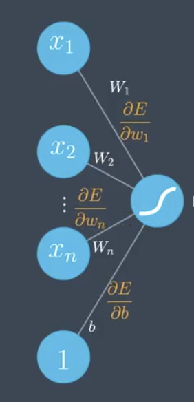
The prediction, error function, and error function gradient follow.
Neural Network
For the neural network, the prediction, error function, and error function gradient are all similar, but the error function gradient is much longer and more complex. It is a huge vector where each element is a partial derivative of the error with respect to each of the weights.
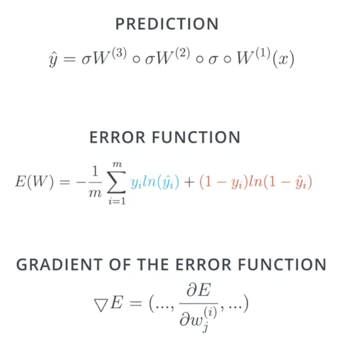
Recall that the prediction is a composition of sigmoids and matrix multiplications. The prediction, weight matrices, and error gradient vector are shown below.
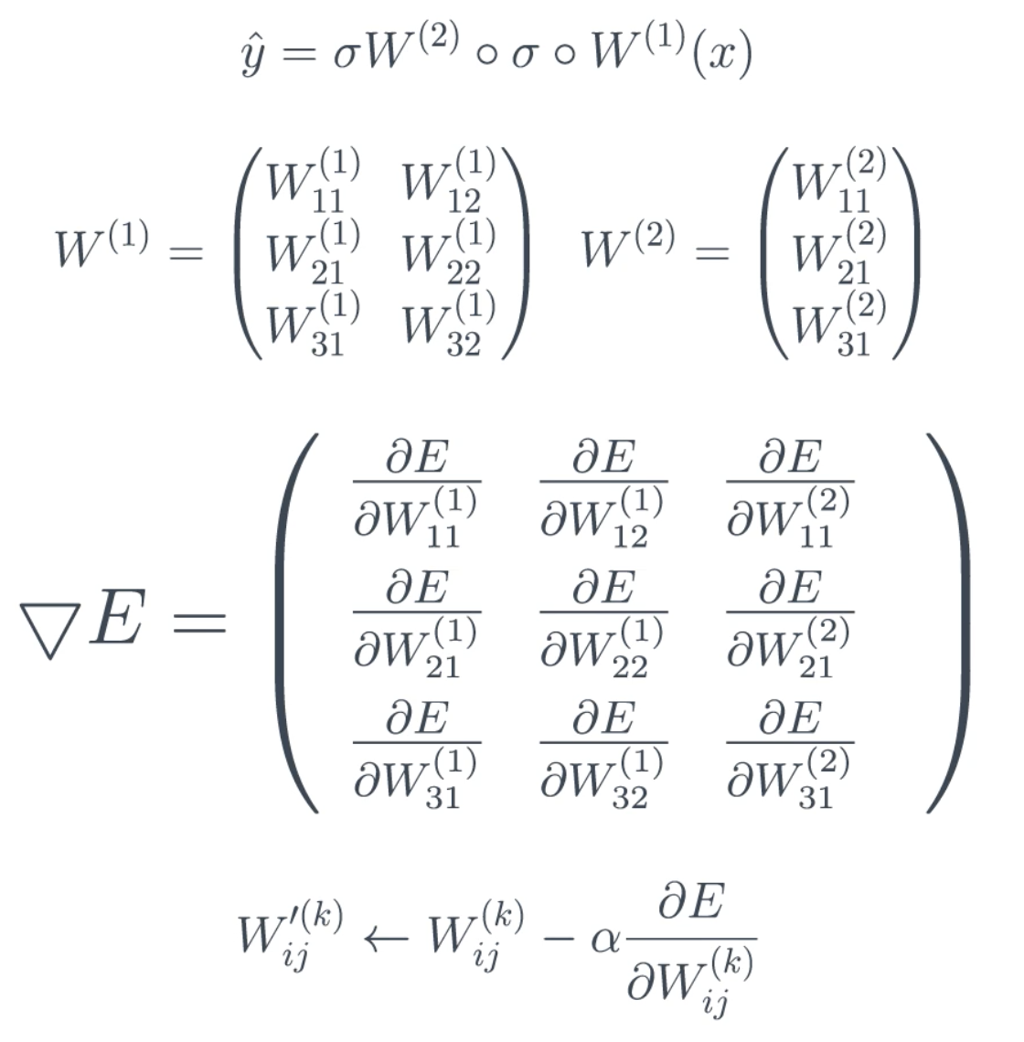
Gradient descent just takes each weight, ${w'}_{ij}^k$, and updates it by adding the learning rate times the partial derivative of $E$ with respect to that same weight. The result is a whole new model.
Chain Rule
The chain rule will be important in calculating the derivatives in order to update the model weights, as outlined above.
Suppose that we have a function $A=f(x)$ and further suppose that a different function B is made by composing a different function, $g$ with $f(x)$ so that $B=g \circ f(x)$. The chain rule gives the following.
$$\frac{\partial B}{\partial x} = \frac{\partial B}{\partial A} \frac{\partial A}{\partial x}$$
What this means is that when composing functions, the derivatives just multiply. This is important because feedforwarding consists of composing a bunch of functions. And, backpropagating is taking the derivative at each piece. So, in order to perform backpropagation we will just multiply several partial derivatives to get what we need.
Calculating the Gradient
Recall the following notation:
- $W^{(2)}$ - indicates the weight belongs to the second layer.
- $W_{12}$ - indicates the weight is between the first node in the layer that is the input to the edge, and the second node in that layer that is the output to the edge.
- $W_{31}$ and $W_{32}$ - the bias terms, written this way for convenience.
Calculate Feedforward
$$h_1 = W_{11}^{(1)} x_1 + W_{21}^{(1)} x_2 + W_{31}^{(1)}$$ $$h_2 = W_{12}^{(1)} x_1 + W_{22}^{(1)} x_2 + W_{32}^{(1)}$$ $$h = W_{11}^{(2)} \sigma (h_1) + W_{21}^{(2)} \sigma (h_2) + W_{31}^{(1)}$$ $$\hat{y} = \sigma (h)$$
Written in more compact notation:
$$\hat{y} = \sigma \circ W^{(2)} \circ \sigma \circ W^{(1)}(x)$$
Calculate Backpropagation
Now calculate more explicit formulae for backpropagation, the exact opposite of feed forward.
To begin, recall that the the error function is a function of the prediction, $\hat{y}$.
$$E(W) = -\frac{1}{m} \sum_{i=1}^m y_i ln(\hat{y}_i) + (1-y_i)ln(1-\hat{y}_i)$$
Since the prediction is itself a function of the weights…
$$E(W) = E(W_{11}^{(1)}, W_{12}^{(1)}, …, W_{31}^{(2)})$$
…the gradient is just the vector formed by the all the partial derivatives of $E$ with respect to each of the weights, $W$.
$$\nabla E = (\frac{\partial E}{\partial W_{11}^{(1)}},…,\frac{\partial E}{\partial W_{31}^{(2)}})$$
Since the prediction is simply a composition of functions, by the chain rule, we know that the derivative of $E$ with respect to one of the weights, $W$, is the product of all the partial derivatives. The fact that we can calculate the derivative of such a complicated composition function by just multiplying four partial derivatives is remarkable.
$$\frac{\partial E}{\partial W_{11}^{(1)}} = \frac{\partial E}{\partial \hat{y}} \frac{\partial \hat{y}}{\partial h} \frac{\partial h}{\partial h_1} \frac{\partial h_1}{\partial W_{11}^{(1)}}$$
Recall that we have already calculated the first one.
$$\frac{\partial E}{\partial \hat{y}}=\hat{y}-y$$
To calculate the next one, we zoom in and focus on just one layer of the network.
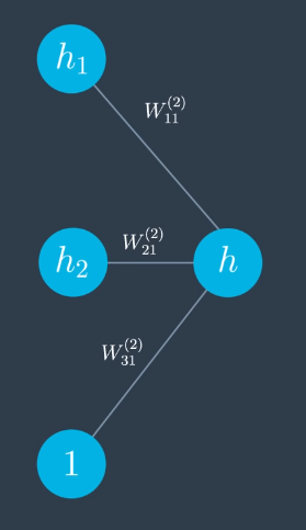
$$h = W_{11}^{(2)} \sigma (h_1) + W_{21}^{(2)} \sigma (h_2) + W_{31}^{(2)}$$
$$\frac{\partial h}{\partial h_1} = W_{11}^{(2)} \sigma (h_1) [1-\sigma(h_1)]$$
To calculate the other partial derivatives, repeat this process.
Note that taking the partial derivative above requires taking the derivative of the sigmoid function, the derivation of which is shown below.
$$\sigma ' (x) = \frac{\partial}{\partial x} \frac{1}{1+e^{-x}}$$ $$= \frac{e^{-x}}{(1+e^{-x})^2}$$ $$=\frac{1}{1+e^{-x}} \times \frac{e^{-x}}{1+e^{-x}}$$ $$=\sigma(x)(1-\sigma(x))$$