Backpropagation

Backpropagation is fundamental to deep learning. Though PyTorch and TensorFlow perform backprop for its users, the users should have an in-depth understanding of the algorithm. With that in mind, Udacity provided the following extra resources from Andrej Karpathy beyond the notes in its lessons:

• Yes, you should understand backprop
• Lecture from Stanford’s CS231n course

High-Level Overview

Backpropagation is fundamental to how neural networks “learn.” An understanding of it is important if you will be training deep neural networks.

From other notes on feed forward and gradient descent, we know how to calculate the error in the output node. We can use this error with gradient descent to train the weights in between the hidden units and output units.

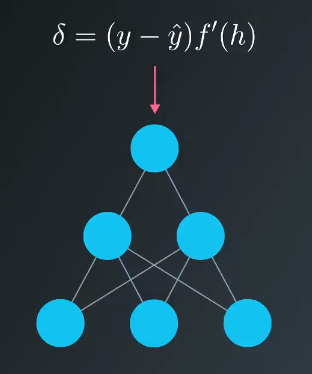
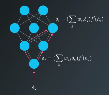
This section focuses on how to calculate the error associated with each of the units in the hidden layer. What we find is that the error associated the hidden units is proportional to the error in the output layer times the weight between the units. This is intuitive because the units with a stronger connection to the output node are going to contribute more error to the final output.

This can be thought of as flipping the network over and using the error as the input.

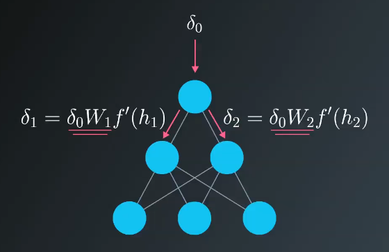
The process is similar if there are more layers; you just keep backpropagating the error to the additional layers, as required.

Mathematics of Backpropagation

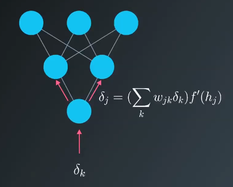
Suppose that in the output layer of a 3 layer neural network, you have errors $\delta_k^o$ attributed to each output unit $k$. The error attributed to hidden unit $j$ is the output errors, scaled by the weights between the output and hidden layers.

$$\delta_j^k = \sum W_{jk} \delta _k^o f'(h_j)$$

The gradient descent step is the same as before but with the addition of new errors

$$\Delta_{ij} = \eta \delta_j^h x_i$$

where $w_{ij}$ are the weights between inputs and hidden layer, and $x_i$ are input unit values. That form holds for however many layers there are. The weight steps are given by

$$\Delta w_{pq} = \eta \delta_{output} V_{in}$$

The output error, $\delta_{output}$, is obtained by propagating the error backwards from higher layers. The input values, $V_{in}$, are the inputs to the layer. For example, the inputs to the output layer would be the hidden layer activations.

Practical Example

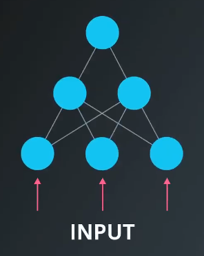
Consider the following two-layer neural network (bottom layer are inputs, shown as nodes, so referred to as a two-layer network here). There are two input values, one hidden unit, and one output unit. The hidden and output units use sigmoid activations.

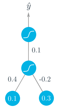
Assume the target is $y=1$. First, calculate the forward pass through the hidden unit

$$h = \sum_i w_i x_i = (0.1 \times 0.4) - (0.2 \times 0.3) = -0.02$$

$$a = f(h) = sigmoid(-0.02) = 0.495$$

This output of the hidden unit is used as the input to the output unit. Then, the output of the network is

$$\hat{y} = f(W \times a) = sigmoid(0.1 \times 0.495) = 0.512$$

Now, start a backwards pass to calculate the weight updates for the layers. Recall the derivative of the sigmoid function: $f'(W \times a) = f(W \times a)(1 - f(W \times a))$. Then the error term for the output is

$$\delta^O = (y-\hat{y})f'(W \times a) = (1 - 0.512) \times 0.512 \times (1-0.512) = 0.122$$

Next, calculate the errror term for the hidden unit with backpropagation. For the hidden unit error term, $\delta_j^h = \sum_k W_{jk} \delta_k^O f'(h_j)$. Since there is one hidden unit and one output unit this is simple.

$$\delta^h = W \delta^O f'(h) = 0.1 \times 0.122 \times 0.495 \times (1 - 0.495) = 0.003$$

Now, caluclate the gradient descent steps. The hidden to output weight step follows:

$$\Delta W = \eta \delta^O a = 0.5 \times 0.122 \times 0.495 = 0.0302$$

Then, for the input to hidden weights:

$$\Delta w_i = \eta \delta^h x_i = (0.5 \times 0.003 \times 0.1, 0.5 \times 0.003 \times 0.3) = (0.00015, 0.00045)$$

Sigmoid Function Impact

The maximum derivative of the sigmoid function is 0.25, so the errors in the output get reduced by at least 75%. Errors in the hidden layer are scaled down by at least 93.75%. So, if there are a lot of layers, using a sigmoid activation function will reduce the weight steps to tiny values in leayers near the input.

This is called the vanishing gradient problem. There are other activation functions that perform better than the sigmoid in in this regard and are more commonly used in today’s neural networks.