Neural Network Architecture
Deep learning networks tend to be massive with dozens or hundreds of layers, that’s where the term “deep” comes from. Its possible to build deep neural networks manually using tensors directly, but in general it’s very cumbersome and difficult to implement. PyTorch has a nice module nn that provides a nice way to efficiently build large neural networks.
%matplotlib inline

import numpy as np
import torch

import matplotlib.pyplot as plt
Now we’re going to build a larger network that can solve a (formerly) difficult problem, identifying text in an image. Here we’ll use the MNIST dataset which consists of greyscale handwritten digits. Each image is 28x28 pixels.
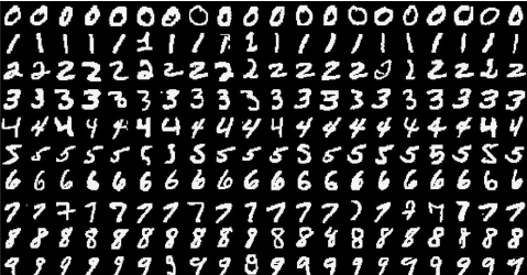
The goal is to build a neural network that can take one of these images and predict the digit in the image.
First up, we need to get our dataset. This is provided through the torchvision package. The code below will download the MNIST dataset, then create training and test datasets for us.
from torchvision import datasets, transforms

# Define a transform to normalize the data
transform = transforms.Compose([transforms.ToTensor(),
                                transforms.Normalize((0.5,), (0.5,)),
                               ])

# Download and load the training data
trainset = datasets.MNIST('~/.pytorch/MNIST_data/',
                          download=True,
                          train=True,
                          transform=transform)
trainloader = torch.utils.data.DataLoader(trainset,
                                          batch_size=64,
                                          shuffle=True)
We have the training data loaded into trainloader and we make that an iterator with iter(trainloader). Later, we’ll use this to loop through the dataset for training, like
for image, label in trainloader:
    ## do things with images and labels
- The
trainloaderwas created with a batch size of 64, andshuffle=True.- The batch size is the number of images we get in one iteration from the data loader and pass through our network, often called a batch.
- And
shuffle=Truetells it to shuffle the dataset every time we start going through the data loader again.
images is just a tensor with size (64, 1, 28, 28). So, 64 images per batch, 1 color channel, and 28x28 images.
dataiter = iter(trainloader)
images, labels = dataiter.next()
print(type(images))
print(images.shape)
print(labels.shape)
<class 'torch.Tensor'>
torch.Size([64, 1, 28, 28])
torch.Size([64])
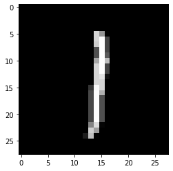
This is what one of the images looks like.
plt.imshow(images[1].numpy().squeeze(),
           cmap='Greys_r');
First, let’s try to build a simple network for this dataset using weight matrices and matrix multiplications. Then, we’ll see how to do it using PyTorch’s nn module which provides a much more convenient and powerful method for defining network architectures.
In fully-connected or dense networks, each unit in one layer is connected to each unit in the next layer. In fully-connected networks, the input to each layer must be a one-dimensional vector (which can be stacked into a 2D tensor as a batch of multiple examples). However, our images are 28x28 2D tensors, so we need to convert them into 1D vectors.
We need to convert the batch of images with shape (64, 1, 28, 28) to a have a shape of (64, 784), 784 is 28 times 28. This is typically called flattening: we flattened the 2D images into 1D vectors.
Flatten the batch of images images.
print('Before reshape:   ' + str(images.shape))
images = images.reshape(64, 784)
print('After reshape:    ' + str(images.shape))
Before reshape:   torch.Size([64, 1, 28, 28])
After reshape:    torch.Size([64, 784])
Here we need 10 output units, one for each digit. We want our network to predict the digit shown in an image, so what we’ll do is calculate probabilities that the image is of any one digit or class. This ends up being a discrete probability distribution over the classes (digits) that tells us the most likely class for the image. That means we need 10 output units for the 10 classes (digits). We’ll see how to convert the network output into a probability distribution next.
Build a multi-layer network with:
- 784 input units,
- 256 hidden units, and
- 10 output units
Use random tensors for the weights and biases. Use a sigmoid activation for the hidden layer and calculate output.
def activation(x):
    return 1/(1+torch.exp(-x))

inputs = images.reshape(images.shape[0], -1)

n_input = images.shape[1] # 784
n_hidden = 256
n_output = 10

W1 = torch.randn(n_input, n_hidden)     # Weights for inputs to hidden layer
W2 = torch.randn(n_hidden, n_output)    # Weights for hidden layer to output layer

B1 = torch.randn((1, n_hidden))         # Bias terms for hidden and output layers
B2 = torch.randn((1, n_output))

hidden = activation(torch.mm(inputs, W1) + B1)
output = activation(torch.mm(hidden, W2) + B2)
print_dict = [('images', images),
              ('W1', W1),
              ('W2', W2),
              ('B1', B1),
              ('B2', B2),
              ('hidden', hidden),
              ('output', output)]
[print(name+':\n\t'+str(tensor.shape)) for name, tensor in print_dict];
images:
	torch.Size([64, 784])
W1:
	torch.Size([784, 256])
W2:
	torch.Size([256, 10])
B1:
	torch.Size([1, 256])
B2:
	torch.Size([1, 10])
hidden:
	torch.Size([64, 256])
output:
	torch.Size([64, 10])
There are 10 outputs for our network. We want to pass in an image to our network and get out a probability distribution over the classes that tells us the likely class(es) the image belongs to. Something that looks like this:
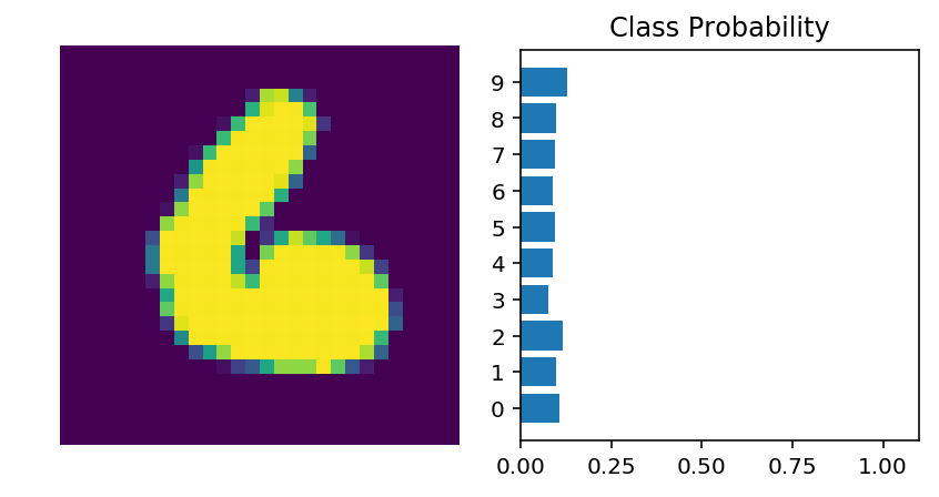
Here we see that the probability for each class is roughly the same. This is representing an untrained network, it hasn’t seen any data yet so it just returns a uniform distribution with equal probabilities for each class.
To calculate this probability distribution, we often use the softmax function. Mathematically this looks like
$$ \Large \sigma(x_i) = \cfrac{e^{x_i}}{\sum_k^K{e^{x_k}}} $$
What this does is squish each input $x_i$ between 0 and 1 and normalizes the values to give you a proper probability distribution where the probabilites sum up to one.
Softmax is implemented in Python as shown below.
dim=1in the parameters of thetorch.sumfunction means to sum across the columns.dim=0would be across the rows..view(-1, 1)reshapes the data to be on one row.
def softmax(x):
    return torch.exp(x)/torch.sum(torch.exp(x), dim=1).view(-1, 1)
probabilities = softmax(output)

# Confirms it has the correct shape
print(probabilities.shape)

# Confirms that the probabilities sum to 1 across the columns
print(probabilities.sum(dim=1))
torch.Size([64, 10])
tensor([1.0000, 1.0000, 1.0000, 1.0000, 1.0000, 1.0000, 1.0000, 1.0000, 1.0000,
        1.0000, 1.0000, 1.0000, 1.0000, 1.0000, 1.0000, 1.0000, 1.0000, 1.0000,
        1.0000, 1.0000, 1.0000, 1.0000, 1.0000, 1.0000, 1.0000, 1.0000, 1.0000,
        1.0000, 1.0000, 1.0000, 1.0000, 1.0000, 1.0000, 1.0000, 1.0000, 1.0000,
        1.0000, 1.0000, 1.0000, 1.0000, 1.0000, 1.0000, 1.0000, 1.0000, 1.0000,
        1.0000, 1.0000, 1.0000, 1.0000, 1.0000, 1.0000, 1.0000, 1.0000, 1.0000,
        1.0000, 1.0000, 1.0000, 1.0000, 1.0000, 1.0000, 1.0000, 1.0000, 1.0000,
        1.0000])
Building networks with PyTorch
PyTorch provides a module nn that makes building networks much simpler.
The network implemented below has the same setup as the network implemented directly with tensors, above. Namely:
- 784 inputs,
- 256 hidden units,
- 10 output units and a
- softmax output.
from torch import nn
class Network(nn.Module):
    def __init__(self):
        super().__init__()

        self.hidden = nn.Linear(784, 256) # Inputs to hidden layer linear transformation
        self.output = nn.Linear(256, 10)  # Output layer, 10 units - one for each digit

        self.sigmoid = nn.Sigmoid()       # Define sigmoid activation and softmax output
        self.softmax = nn.Softmax(dim=1)

    def forward(self, x):
        x = self.hidden(x)                # Pass the input tensor through each of our operations
        x = self.sigmoid(x)
        x = self.output(x)
        x = self.softmax(x)

        return x
Let’s go through this bit by bit.
class Network(nn.Module):
Here we’re inheriting from nn.Module. Combined with super().__init__() this creates a class that tracks the architecture and provides a lot of useful methods and attributes. It is mandatory to inherit from nn.Module when you’re creating a class for your network. The name of the class itself can be anything.
self.hidden = nn.Linear(784, 256)
This line creates a module for a linear transformation, $x\mathbf{W} + b$, with 784 inputs and 256 outputs and assigns it to self.hidden. The module automatically creates the weight and bias tensors which we’ll use in the forward method. You can access the weight and bias tensors once the network (net) is created with net.hidden.weight and net.hidden.bias.
self.output = nn.Linear(256, 10)
Similarly, this creates another linear transformation with 256 inputs and 10 outputs.
self.sigmoid = nn.Sigmoid()
self.softmax = nn.Softmax(dim=1)
Here I defined operations for the sigmoid activation and softmax output. Setting dim=1 in nn.Softmax(dim=1) calculates softmax across the columns.
def forward(self, x):
PyTorch networks created with nn.Module must have a forward method defined. It takes in a tensor x and passes it through the operations you defined in the __init__ method.
x = self.hidden(x)
x = self.sigmoid(x)
x = self.output(x)
x = self.softmax(x)
Here the input tensor x is passed through each operation and reassigned to x. We can see that the input tensor goes:
- through the hidden layer,
- then a sigmoid function,
- then the output layer, and
- finally the softmax function.
It doesn’t matter what you name the variables here, as long as the inputs and outputs of the operations match the network architecture you want to build. The order in which you define things in the __init__ method doesn’t matter, but you’ll need to sequence the operations correctly in the forward method.
Now we can create a Network object.
model = Network()      # Create the network and look at it's text representation
model
Network(
  (hidden): Linear(in_features=784, out_features=256, bias=True)
  (output): Linear(in_features=256, out_features=10, bias=True)
  (sigmoid): Sigmoid()
  (softmax): Softmax(dim=1)
)
You can define the network somewhat more concisely and clearly using the torch.nn.functional module. This is the most common way you’ll see networks defined as many operations are simple element-wise functions. We normally import this module as F, import torch.nn.functional as F.
import torch.nn.functional as F

class Network(nn.Module):
    def __init__(self):
        super().__init__()
        self.hidden = nn.Linear(784, 256)      # Inputs to hidden layer linear transformation
        self.output = nn.Linear(256, 10)       # Output layer, 10 units - one for each digit

    def forward(self, x):
        x = F.sigmoid(self.hidden(x))          # Hidden layer with sigmoid activation
        x = F.softmax(self.output(x), dim=1)   # Output layer with softmax activation

        return x
Activation functions
So far we’ve only been looking at the sigmoid activation function, but in general any function can be used as an activation function. The only requirement is that for a network to approximate a non-linear function, the activation functions must be non-linear. Here are a few more examples of common activation functions:
- Tanh (hyperbolic tangent), and
- ReLU (rectified linear unit).
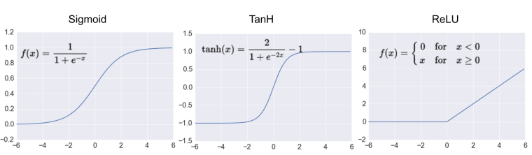
In practice, the ReLU function is used almost exclusively as the activation function for hidden layers.
Another Example
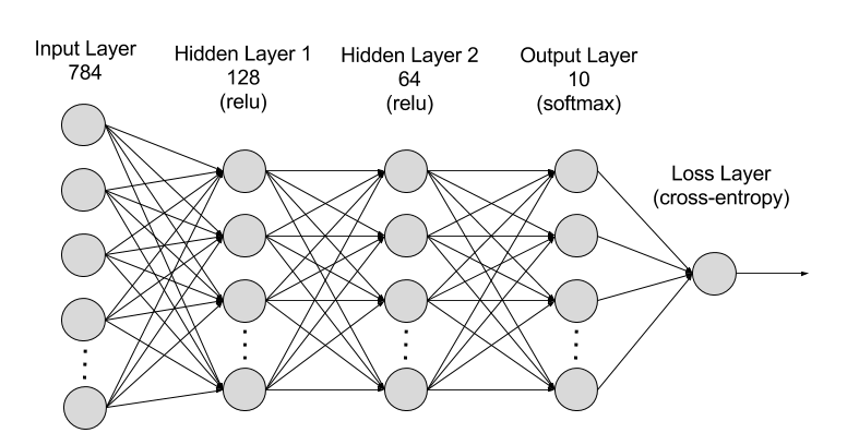
Create a network with:
- 784 input units,
- a hidden layer with 128 units and a ReLU activation, then
- a hidden layer with 64 units and a ReLU activation, and finally
- an output layer with 10 units and a softmax activation as shown above.
You can use a ReLU activation with the nn.ReLU module or F.relu function.
It’s good practice to name your layers by their type of network, for instance ‘fc’ to represent a fully-connected layer.
class Network(nn.Module):
    def __init__(self):
        super().__init__()
        self.fc1 = nn.Linear(784, 128)      # Inputs to hidden layer linear transformation
        self.fc2 = nn.Linear(128, 64)       # Hidden layer
        self.fc3 = nn.Linear(64, 10)        # Output layer, 10 units - one for each digit

    def forward(self, x):
        x = F.relu(self.fc1(x))             # Hidden layer, sigmoid
        x = F.relu(self.fc2(x))             # Hidden layer, sigmoid
        x = F.softmax(self.fc3(x), dim=1)   # Output layer, softmax

        return x

model = Network()
model
Network(
  (fc1): Linear(in_features=784, out_features=128, bias=True)
  (fc2): Linear(in_features=128, out_features=64, bias=True)
  (fc3): Linear(in_features=64, out_features=10, bias=True)
)
Initializing weights and biases
The weights and such are automatically initialized. But, it’s possible to customize how they are initialized. The weights and biases are tensors attached to each layer. They are accessible with model.fc1.weight for instance.
print(model.fc1.weight)
print(model.fc1.bias)
Parameter containing:
tensor([[-2.4966e-03,  1.1749e-02, -2.6093e-02,  ..., -1.2360e-02,
          3.5630e-02,  4.7725e-03],
        [-3.2441e-02,  3.2651e-02,  3.3655e-02,  ...,  2.1452e-02,
          2.7882e-02, -1.6112e-02],
        [ 2.0714e-02,  3.3352e-02,  2.6289e-02,  ...,  1.2436e-02,
          7.4691e-03, -2.8511e-02],
        ...,
        [-2.3080e-02,  3.1245e-04,  2.9845e-02,  ..., -4.6726e-05,
         -2.9866e-02,  2.5208e-02],
        [-1.8899e-02, -3.0683e-03,  2.3156e-02,  ..., -3.1593e-02,
          4.9126e-03,  1.1597e-02],
        [ 2.6959e-02,  3.0315e-02, -9.8074e-03,  ...,  1.2507e-02,
          1.9535e-02, -3.6948e-03]], requires_grad=True)
Parameter containing:
tensor([-0.0314,  0.0139, -0.0152, -0.0202, -0.0128, -0.0184,  0.0262, -0.0326,
        -0.0210, -0.0083, -0.0181,  0.0028,  0.0179,  0.0103, -0.0191, -0.0230,
        -0.0085, -0.0127, -0.0158,  0.0253,  0.0212, -0.0154, -0.0282, -0.0323,
        -0.0216,  0.0086, -0.0186, -0.0188,  0.0352,  0.0156,  0.0009,  0.0058,
        -0.0006, -0.0225, -0.0197, -0.0341,  0.0294, -0.0116,  0.0263, -0.0239,
         0.0076, -0.0012,  0.0020, -0.0191,  0.0138, -0.0180,  0.0043,  0.0084,
        -0.0356,  0.0079,  0.0070, -0.0161, -0.0103,  0.0211,  0.0177,  0.0269,
        -0.0246, -0.0096, -0.0148,  0.0278, -0.0135, -0.0142, -0.0302, -0.0037,
         0.0084,  0.0009,  0.0287,  0.0035, -0.0058, -0.0321, -0.0162, -0.0356,
        -0.0224,  0.0335, -0.0286,  0.0269, -0.0078,  0.0168, -0.0272,  0.0254,
        -0.0283, -0.0113, -0.0330,  0.0342, -0.0207, -0.0336,  0.0200, -0.0010,
        -0.0093, -0.0112, -0.0112, -0.0097,  0.0321,  0.0251,  0.0282,  0.0119,
         0.0184,  0.0010, -0.0356, -0.0156,  0.0138,  0.0337,  0.0196,  0.0030,
         0.0334,  0.0270,  0.0108, -0.0117,  0.0167,  0.0022,  0.0257,  0.0079,
         0.0010,  0.0024, -0.0037, -0.0334, -0.0114,  0.0014, -0.0330, -0.0053,
         0.0326, -0.0321, -0.0310,  0.0242,  0.0274, -0.0123, -0.0263,  0.0321],
       requires_grad=True)
For custom initialization, we want to modify these tensors in place. These are actually autograd Variables, so we need to get back the actual tensors with model.fc1.weight.data. Once we have the tensors, we can fill them with zeros (for biases) or random normal values.
- Set biases to all zeros
model.fc1.bias.data.fill_(0)
tensor([0., 0., 0., 0., 0., 0., 0., 0., 0., 0., 0., 0., 0., 0., 0., 0., 0., 0., 0., 0., 0., 0., 0., 0.,
        0., 0., 0., 0., 0., 0., 0., 0., 0., 0., 0., 0., 0., 0., 0., 0., 0., 0., 0., 0., 0., 0., 0., 0.,
        0., 0., 0., 0., 0., 0., 0., 0., 0., 0., 0., 0., 0., 0., 0., 0., 0., 0., 0., 0., 0., 0., 0., 0.,
        0., 0., 0., 0., 0., 0., 0., 0., 0., 0., 0., 0., 0., 0., 0., 0., 0., 0., 0., 0., 0., 0., 0., 0.,
        0., 0., 0., 0., 0., 0., 0., 0., 0., 0., 0., 0., 0., 0., 0., 0., 0., 0., 0., 0., 0., 0., 0., 0.,
        0., 0., 0., 0., 0., 0., 0., 0.])
- Sample from random normal with standard dev = 0.01
model.fc1.weight.data.normal_(std=0.01)
tensor([[-0.0077, -0.0016,  0.0113,  ..., -0.0131, -0.0185, -0.0128],
        [ 0.0036, -0.0091,  0.0038,  ...,  0.0035,  0.0069,  0.0023],
        [-0.0146,  0.0030, -0.0030,  ..., -0.0175, -0.0054,  0.0112],
        ...,
        [ 0.0137, -0.0007,  0.0125,  ...,  0.0063, -0.0008, -0.0072],
        [-0.0026, -0.0068,  0.0001,  ...,  0.0019,  0.0098,  0.0245],
        [-0.0004,  0.0049,  0.0035,  ..., -0.0033,  0.0133, -0.0116]])
Forward pass
Now pass an image into the network.
- Get some data.
- Resize images into a 1D vector. The new shape is (batch size, color channels, image pixels).
- Or, use
images.resize_(images.shape[0], 1, 784)to automatically get batch size.
- Or, use
- Forward pass.
The following is a helper function to view and image and it’s predicted classes.
def view_classify(img, ps):
    ps = ps.data.numpy().squeeze()

    fig, (ax1, ax2) = plt.subplots(figsize=(6,9), ncols=2)
    ax1.imshow(img.resize_(1, 28, 28).numpy().squeeze())
    ax1.axis('off')
    ax2.barh(np.arange(10), ps)
    ax2.set_aspect(0.1)
    ax2.set_yticks(np.arange(10))
    ax2.set_yticklabels(np.arange(10))
    ax2.set_title('Class Probability')
    ax2.set_xlim(0, 1.1)

    plt.tight_layout()
# Grab some data
dataiter = iter(trainloader)
images, labels = dataiter.next()

# Resize images
images.resize_(images.shape[0], 1, 784)

# Forward pass through the network
img_idx = 0
ps = model.forward(images[img_idx,:])

img = images[img_idx]
view_classify(img.view(1, 28, 28), ps)
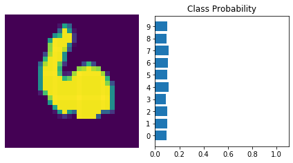
The network has basically no idea what this digit is. This is because the network hasn’t been trained yet. All the weights are currently random.
Using nn.Sequential
PyTorch provides a convenient way to build networks like this where a tensor is passed sequentially through operations, nn.Sequential (documentation). Using this to build the equivalent network:
# Hyperparameters for our network
input_size = 784
hidden_sizes = [128, 64]
output_size = 10
# Build a feed-forward network
model = nn.Sequential(nn.Linear(input_size, hidden_sizes[0]),
nn.ReLU(),
nn.Linear(hidden_sizes[0], hidden_sizes[1]),
nn.ReLU(),
nn.Linear(hidden_sizes[1], output_size),
nn.Softmax(dim=1))
print(model)
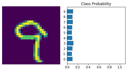
# Forward pass through the network
images, labels = next(iter(trainloader))
images.resize_(images.shape[0], 1, 784)
ps = model.forward(images[0,:])
# Display output
view_classify(images[0].view(1, 28, 28), ps)
Sequential(
  (0): Linear(in_features=784, out_features=128, bias=True)
  (1): ReLU()
  (2): Linear(in_features=128, out_features=64, bias=True)
  (3): ReLU()
  (4): Linear(in_features=64, out_features=10, bias=True)
  (5): Softmax(dim=1)
)
Here the model is the same as before:
- 784 input units,
- a hidden layer with 128 units, ReLU activation,
- 64 unit hidden layer, another ReLU,
- then the output layer with 10 units, and the softmax output.
The operations are available by passing in the appropriate index. For example, to get first Linear operation and look at the weights, you’d use model[0].
print(model[0])
model[0].weight
Linear(in_features=784, out_features=128, bias=True)


Parameter containing:
tensor([[-0.0250,  0.0118,  0.0305,  ..., -0.0200,  0.0032,  0.0231],
        [-0.0143,  0.0034, -0.0200,  ...,  0.0351,  0.0195, -0.0356],
        [-0.0275, -0.0216, -0.0183,  ..., -0.0320, -0.0176,  0.0347],
        ...,
        [-0.0277,  0.0050, -0.0249,  ...,  0.0260, -0.0145,  0.0185],
        [-0.0016,  0.0016, -0.0338,  ..., -0.0065,  0.0274,  0.0065],
        [-0.0344,  0.0274,  0.0311,  ...,  0.0318,  0.0021, -0.0350]],
       requires_grad=True)
You can also pass in an OrderedDict to name the individual layers and operations, instead of using incremental integers. Note that dictionary keys must be unique, so each operation must have a different name.
from collections import OrderedDict
model = nn.Sequential(OrderedDict([
    ('fc1', nn.Linear(input_size, hidden_sizes[0])),
    ('relu1', nn.ReLU()),
    ('fc2', nn.Linear(hidden_sizes[0], hidden_sizes[1])),
    ('relu2', nn.ReLU()),
    ('output', nn.Linear(hidden_sizes[1], output_size)),
    ('softmax', nn.Softmax(dim=1))]))
model
Sequential(
  (fc1): Linear(in_features=784, out_features=128, bias=True)
  (relu1): ReLU()
  (fc2): Linear(in_features=128, out_features=64, bias=True)
  (relu2): ReLU()
  (output): Linear(in_features=64, out_features=10, bias=True)
  (softmax): Softmax(dim=1)
)
Now the layers are accessible by integer or the name.
print(model[0])
print(model.fc1)
Linear(in_features=784, out_features=128, bias=True)
Linear(in_features=784, out_features=128, bias=True)
Copyright © 2018 Udacity