Classifying Fashion MNIST
This example uses the Fashion-MNIST dataset, a drop-in replacement for the MNIST dataset. MNIST is actually quite trivial with neural networks. Its possible to easily achieve better than 97% accuracy. Fashion-MNIST is a set of 28x28 greyscale images of clothes. It’s more complex than MNIST, so it’s a better representation of the actual performance of your network, and a better representation of datasets used in the real world.
First, load the dataset through torchvision.
import torch
from torchvision import datasets, transforms

# Define a transform to normalize the data
transform = transforms.Compose([transforms.ToTensor(),
                                transforms.Normalize((0.5,), (0.5,))])
# Download and load the training data
trainset = datasets.FashionMNIST('~/.pytorch/F_MNIST_data/',
                                 download=True,
                                 train=True,
                                 transform=transform)
trainloader = torch.utils.data.DataLoader(trainset,
                                          batch_size=64,
                                          shuffle=True)

# Download and load the test data
testset = datasets.FashionMNIST('~/.pytorch/F_MNIST_data/',
                                download=True,
                                train=False,
                                transform=transform)
testloader = torch.utils.data.DataLoader(testset,
                                         batch_size=64,
                                         shuffle=True)
The following is a helper function to print one of the images.
import matplotlib.pyplot as plt
import numpy as np

def imshow(image, ax=None, title=None, normalize=True):
    if ax is None:
        fig, ax = plt.subplots()
    image = image.numpy().transpose((1, 2, 0))

    if normalize:
        mean = np.array([0.485, 0.456, 0.406])
        std = np.array([0.229, 0.224, 0.225])
        image = std * image + mean
        image = np.clip(image, 0, 1)

    ax.imshow(image)
    ax.spines['top'].set_visible(False)
    ax.spines['right'].set_visible(False)
    ax.spines['left'].set_visible(False)
    ax.spines['bottom'].set_visible(False)
    ax.tick_params(axis='both', length=0)
    ax.set_xticklabels('')
    ax.set_yticklabels('')

    return ax
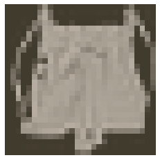
Here we can see one of the images.
image, label = next(iter(trainloader))
imshow(image[0,:]);
Defining the Network Architecture
Defining the network architecture, IE, “build the network.”
As with MNIST, each image is 28x28 which is a total of 784 pixels, and there are 10 classes. Notes regarding recommended network architecture for fashion-mnist:
- At least one hidden layer is necessary.
- ReLU activations are recommended for the layers
- Logits or log-softmax are recommended from the forward pass.
For straightforward comparison with results on the standard MNIST, use the same network setup.
from torch import nn

model = nn.Sequential(nn.Linear(784, 128),
                      nn.ReLU(),
                      nn.Linear(128, 64),
                      nn.ReLU(),
                      nn.Linear(64, 10),
                      nn.LogSoftmax(dim=1))
Train the network
Now, create the network and train it.
First, define:
- the criterion (something like
nn.CrossEntropyLoss) and - the optimizer (typically
optim.SGDoroptim.Adam).
from torch import optim

criterion = nn.NLLLoss()
optimizer = optim.SGD(model.parameters(),
                      lr=0.003)
Then, train the network. The training pass is a fairly straightforward process:
- Make a forward pass through the network to get the logits
- Use the logits to calculate the loss
- Perform a backward pass through the network with
loss.backward()to calculate the gradients - Take a step with the optimizer to update the weights
A training loss rate below 0.4 should be possible on the dataset.
epoch = 1
while True:
    running_loss = 0
    for images, labels in trainloader:
        # Flatten MNIST images into a 784 long vector
        images = images.view(images.shape[0], -1)

        optimizer.zero_grad()

        output = model(images)
        loss = criterion(output, labels)
        loss.backward()
        optimizer.step()

        running_loss += loss.item()

    training_loss = running_loss/len(trainloader)
    print("Epoch, Loss:    {:2}, {:1.3}".format(epoch, training_loss))
    epoch += 1

    if training_loss < 0.4:
        break
Epoch, Loss:     1, 1.65
Epoch, Loss:     2, 0.834
Epoch, Loss:     3, 0.665
Epoch, Loss:     4, 0.6
Epoch, Loss:     5, 0.559
Epoch, Loss:     6, 0.531
Epoch, Loss:     7, 0.509
Epoch, Loss:     8, 0.492
Epoch, Loss:     9, 0.479
Epoch, Loss:    10, 0.467
Epoch, Loss:    11, 0.457
Epoch, Loss:    12, 0.449
Epoch, Loss:    13, 0.441
Epoch, Loss:    14, 0.434
Epoch, Loss:    15, 0.428
Epoch, Loss:    16, 0.422
Epoch, Loss:    17, 0.417
Epoch, Loss:    18, 0.412
Epoch, Loss:    19, 0.407
Epoch, Loss:    20, 0.403
Epoch, Loss:    21, 0.398
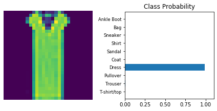
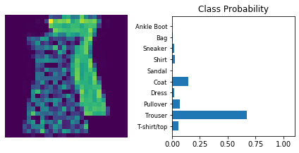
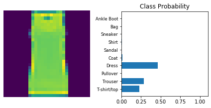
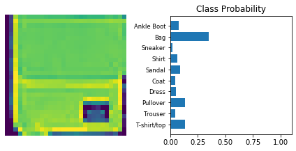
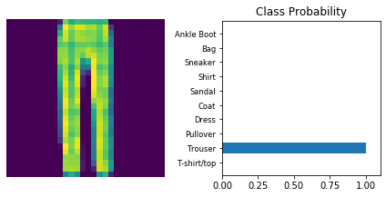
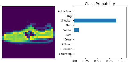
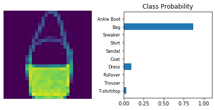
The following is a helper function to print
%matplotlib inline
import matplotlib.pyplot as plt
import numpy as np

def view_classify(img, ps):
    ps = ps.data.numpy().squeeze()

    fig, (ax1, ax2) = plt.subplots(figsize=(6,9), ncols=2)
    ax1.imshow(img.resize_(1, 28, 28).numpy().squeeze())
    ax1.axis('off')
    ax2.barh(np.arange(10), ps)
    ax2.set_aspect(0.1)
    ax2.set_yticks(np.arange(10))
    ax2.set_yticklabels(['T-shirt/top',
                        'Trouser',
                        'Pullover',
                        'Dress',
                        'Coat',
                        'Sandal',
                        'Shirt',
                        'Sneaker',
                        'Bag',
                        'Ankle Boot'], size='small');
    ax2.set_title('Class Probability')
    ax2.set_xlim(0, 1.1)

    plt.tight_layout()
dataiter = iter(testloader)
for _ in range(10):
images, labels = dataiter.next()
img = images[0]
# Convert 2D image to 1D vector
img = img.resize_(1, 784)
# Turn off gradients to speed up this part
with torch.no_grad():
logps = model(img)
# Output of the network are log-probabilities, need to take exponential for probabilities
ps = torch.exp(logps)
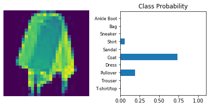
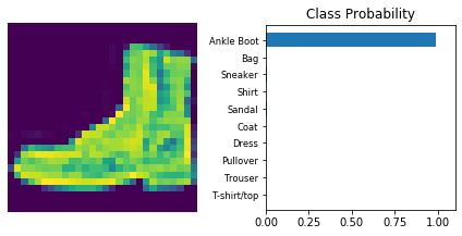
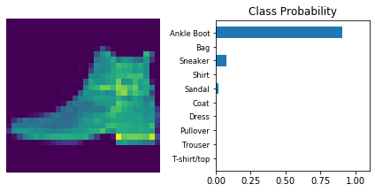
# Plot the image and probabilities
view_classify(img.resize_(1, 28, 28), ps)
Copyright © 2018 Udacity