financial advice. You should do your own research before making any decisions.
Inflation-Adjusted Income Analysis
The goal of this analysis is to take an objective, hard-nosed look at trends in the real-world purchasing power equivalent of the income a typical professional could have earned over the past 5 years. To do so I normalize the nominal income of a typical mid-career professional against the factors below, while also taking into account probable income increases over that time period.
- Consumables, i.e. “Just Getting By” expenses:
- CPI Inflation, (i.e. Cost-of-Living Adjustments)
- Food price changes
- Shelter price changes
- Energy price changes
- CPI Inflation, (i.e. Cost-of-Living Adjustments)
- Scarce Desirable Assets, i.e. “Getting Ahead and Building a Future” purchases:
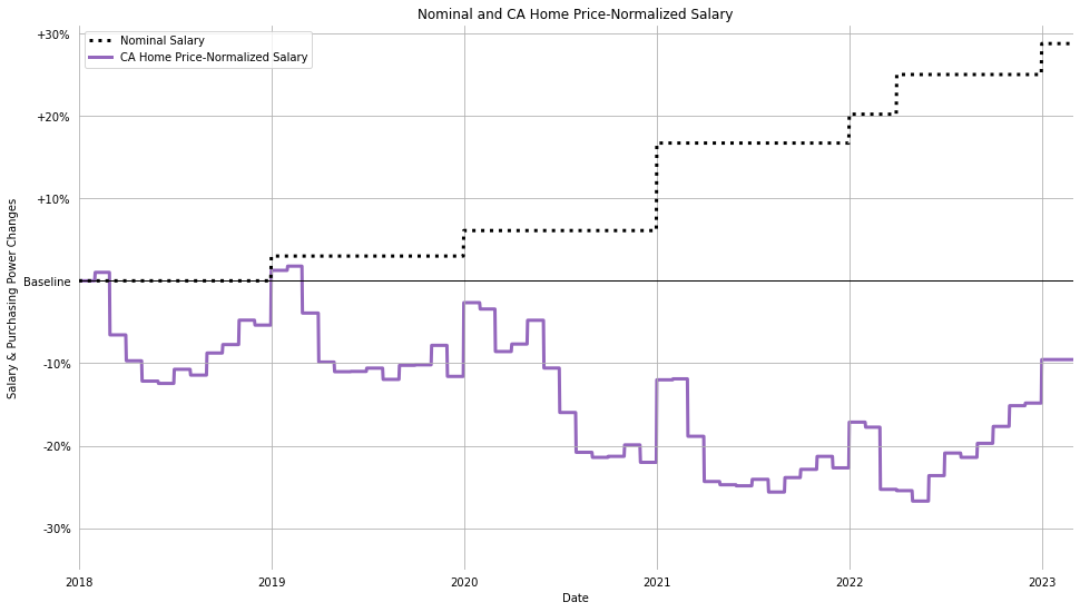
- Median Home price changes
- Gold price changes
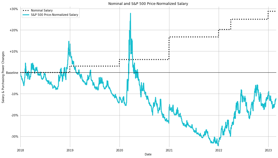
- S&P 500 price changes
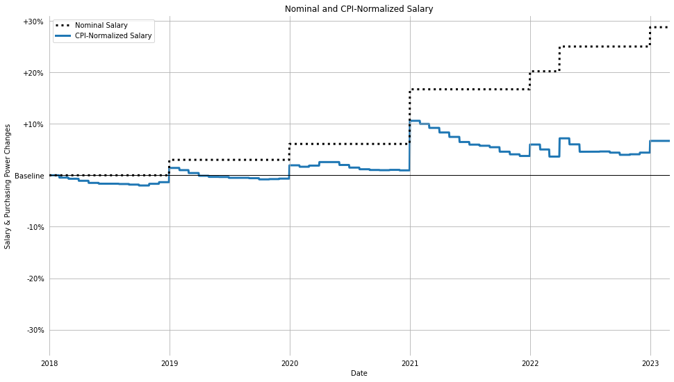
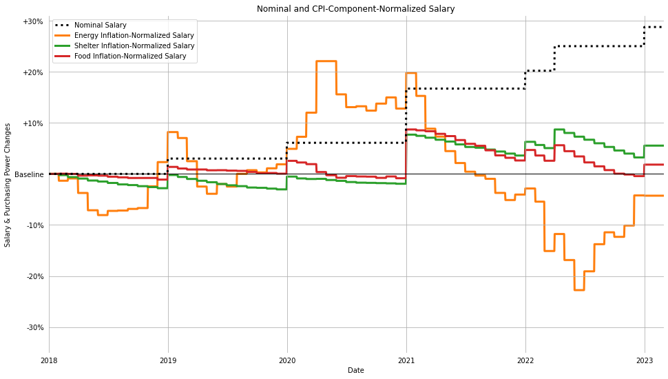
The outcome of this analysis is a set of visuals showing that professionals with even an above-average career trajectory may not be “getting ahead” in real, purchasing power terms the way they may feel they are in nominal, dollar-denominated terms. Specifically, even relatively successful professionals (like those whose salaries increased nearly 30% in 5 years) can purchase:
- only ~6% more “shelter,”
- only ~2% more food,
- ~2% less energy,
- ~10% less home in California,
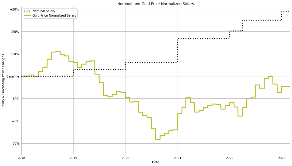
- ~5% less gold, and
- ~13% less of the S&P 500
with their salary than they could at the start of the 5 year period prior to the salary increases. These percentages are taken by comparing the normalized salary in early 2023 to the baseline salary in 2018.
This sense of working as hard as you can to just stay in the same place is not "just you." It is a real phenomena and can be backed up with data.
The root cause is a broken fiat currency.

“Nominal” Income Assumptions
The example assumes the following pay increases. Most years the increase is a standard 3% cost of living adjustment. A 10% performance bonus in 2021 and a one-time special 4% inflation adjustement in April, 2022 is also included.
| Date | Adjustment to Start Period | Cumulative Increase |
|---|---|---|
| 2018-01-01 | N/A | 0% |
| 2019-01-01 | +3% | +3.0% |
| 2020-01-01 | +3% | +6.1% |
| 2021-01-01 | +10% | +16.7% |
| 2022-01-01 | +3% | +20.2% |
| 2022-04-01 | +4% | +25.0% |
| 2023-01-01 | +3% | +28.8% |
Adjustments to Calculate a “Real” Income
Consumer Price Index (CPI) Inflation
The U.S. Bureau of Labor Statistics has a CPI inflation calculator that uses the Consumer Price Index for All Urban Consumers (CPI-U) to calculate changes in the “buying power” of the dollar over time. Using that calculator, the bureau reports, “\$100.00 in January, 2023 has the same buying power as \$82.85 in January, 2018.”
The data is baselined off of a time period from 1982 until 1984. What \$100 could have purchased during the 1982 until 1984 base period, it takes $299.17 to purchase in January, 2023.
Shelter, Food, and Energy Price Changes
The CPI metric relies on pricing data for items in a market basket of goods and services that are important factors in the cost of living for US consumers. Three of these components that may be particularly important are shelter, food, and energy. The data are structurally similar to the data from the CPI Inflation section.
Median Existing California Home Price Changes
Data taken from California Association of Realtors.
Gold Price Changes
Data taken from Index Mundi.
S&P 500 Price Changes
Data taken from investing.com.


Detailed Analysis & Data Manipulation
Set Up Pandas and Data
# Ingore Warning:
# ipykernel_launcher.py:22: UserWarning: FixedFormatter
#should only be used together with FixedLocator
import warnings
warnings.filterwarnings("ignore")

import pandas as pd
import datetime as dt
import matplotlib.pyplot as plt
Income Trajectory Over Time
income_values = {
    'date' : ['2018-01-01', '2019-01-01', '2020-01-01', '2021-01-01',
              '2022-01-01', '2022-04-01', '2023-01-01'],
    'nominal salary' : [100000, 103000, 106090, 116699, 120200, 125008, 128758]
}
i = pd.DataFrame(income_values)

date_range = pd.DataFrame(pd.date_range(dt.datetime(2018, 1, 1),
                                        dt.datetime(2023, 3, 1)),
                          columns=['date'])
date_range['date'] = date_range['date'].astype(str)

i = pd.merge(date_range, i,
             on='date',
             how='left')
i['nominal salary'] = i['nominal salary'].fillna(method='ffill')
i.head(3)
| date | nominal salary | |
|---|---|---|
| 0 | 2018-01-01 | 100000.0 |
| 1 | 2018-01-02 | 100000.0 |
| 2 | 2018-01-03 | 100000.0 |
Consumer Price Index (CPI) Inflation
The methodology employed below is to normalizing the CPI metric to the baseline CPI metric at the start of this analysis on 2018-01-01, which was 247.867. So, the observation on 2023-01-01 of 299.170 would be standardized to roughly 1.21, indicating that things have become roughly 21% “more expensive” in 2023 as compared to 2018.
filepath = 'inflation-adjusted-income-analysis/cpi_columnar_CUUR0000SA0_230308_1.xlsx'
c = (pd.read_excel(filepath,
                   skiprows=11)
     .drop(columns=['Series ID','Unnamed: 4','Unnamed: 5'])
     .rename(columns={'Value' : 'cpi'}))
c = c[(c['Year'].isin([2018, 2019, 2020, 2021, 2022, 2023]))&
      (~c['Period'].isin(['S01','S02']))].reset_index(drop=True)
c['date'] = c['Year'].astype(str) + '-' + c['Period'].str.replace('M','') + '-01'
c = c[['date','cpi']].reset_index(drop=True)
c['norm cpi'] = c['cpi'] / c.iloc[0]['cpi']
c.head(3)
| date | cpi | norm cpi | |
|---|---|---|---|
| 0 | 2018-01-01 | 247.867 | 1.000000 |
| 1 | 2018-02-01 | 248.991 | 1.004535 |
| 2 | 2018-03-01 | 249.554 | 1.006806 |
c.tail(3)
| date | cpi | norm cpi | |
|---|---|---|---|
| 58 | 2022-11-01 | 297.711 | 1.201092 |
| 59 | 2022-12-01 | 296.797 | 1.197404 |
| 60 | 2023-01-01 | 299.170 | 1.206978 |
Shelter Price Inflation
Data is normalized similarly to the previous sections.
filepath = 'inflation-adjusted-income-analysis/shelter_columnar_CUUR0000SAH1_230309_1.xlsx'
s = (pd.read_excel(filepath,
                   skiprows=11)
     .drop(columns=['Series ID','Unnamed: 4','Unnamed: 5'])
     .rename(columns={'Value' : 'shelter infl'}))
s = s[(s['Year'].isin([2018, 2019, 2020, 2021, 2022, 2023]))&
      (~s['Period'].isin(['S01','S02']))].reset_index(drop=True)
s['date'] = s['Year'].astype(str) + '-' + s['Period'].str.replace('M','') + '-01'
s = s[['date','shelter infl']].reset_index(drop=True)
s['norm shelter infl'] = s['shelter infl'] / s.iloc[0]['shelter infl']
s.head(3)
| date | shelter infl | norm shelter infl | |
|---|---|---|---|
| 0 | 2018-01-01 | 302.928 | 1.000000 |
| 1 | 2018-02-01 | 303.653 | 1.002393 |
| 2 | 2018-03-01 | 304.847 | 1.006335 |
s.tail(3)
| date | shelter infl | norm shelter infl | |
|---|---|---|---|
| 58 | 2022-11-01 | 364.195 | 1.202249 |
| 59 | 2022-12-01 | 366.868 | 1.211073 |
| 60 | 2023-01-01 | 369.585 | 1.220042 |
Food Price Inflation
Data is normalized similarly to the previous section.
filepath = 'inflation-adjusted-income-analysis/food_columnar_CUUR0000SAF1_230309_1.xlsx'
f = (pd.read_excel(filepath,
                   skiprows=11)
     .drop(columns=['Unnamed: 4', 'Unnamed: 5', 'Unnamed: 6',
                    'Unnamed: 7', 'Unnamed: 8', 'Unnamed: 9',
                    'Unnamed: 10', 'Unnamed: 11', 'Unnamed: 12'])
     .rename(columns={'Observation Value' : 'food infl'}))
f = f[(f['Year'].isin([2018, 2019, 2020, 2021, 2022, 2023]))&
      (~f['Period'].isin(['S01','S02']))].reset_index(drop=True)
f['date'] = f['Year'].astype(str) + '-' + f['Period'].str.replace('M','') + '-01'
f = f[['date','food infl']].reset_index(drop=True)
f['norm food infl'] = f['food infl'] / f.iloc[0]['food infl']
f.head(3)
| date | food infl | norm food infl | |
|---|---|---|---|
| 0 | 2018-01-01 | 252.361 | 1.000000 |
| 1 | 2018-02-01 | 252.266 | 0.999624 |
| 2 | 2018-03-01 | 252.370 | 1.000036 |
f.tail(3)
| date | food infl | norm food infl | |
|---|---|---|---|
| 58 | 2022-11-01 | 315.857 | 1.251608 |
| 59 | 2022-12-01 | 316.839 | 1.255499 |
| 60 | 2023-01-01 | 319.136 | 1.264601 |
Energy Price Inflation
Data is normalized similarly to the previous sections.
filepath = 'inflation-adjusted-income-analysis/energy_columnar_CUUR0000SA0E_230310_1.xlsx'
e = (pd.read_excel(filepath,
                   skiprows=11)
     .drop(columns=['Series ID','Unnamed: 4','Unnamed: 5'])
     .rename(columns={'Value' : 'energy infl'}))
e = e[(e['Year'].isin([2018, 2019, 2020, 2021, 2022, 2023]))&
      (~e['Period'].isin(['S01','S02']))].reset_index(drop=True)
e['date'] = e['Year'].astype(str) + '-' + e['Period'].str.replace('M','') + '-01'
e = e[['date','energy infl']].reset_index(drop=True)
e['norm energy infl'] = e['energy infl'] / e.iloc[0]['energy infl']
e.head(3)
| date | energy infl | norm energy infl | |
|---|---|---|---|
| 0 | 2018-01-01 | 210.663 | 1.000000 |
| 1 | 2018-02-01 | 213.519 | 1.013557 |
| 2 | 2018-03-01 | 212.554 | 1.008976 |
e.tail(3)
| date | energy infl | norm energy infl | |
|---|---|---|---|
| 58 | 2022-11-01 | 292.953 | 1.390624 |
| 59 | 2022-12-01 | 274.937 | 1.305103 |
| 60 | 2023-01-01 | 283.330 | 1.344944 |
Home Price Inflation
Data is normalized similarly to the previous sections.
filepath = 'inflation-adjusted-income-analysis/MedianPricesofExistingDetachedHomes.xlsx'
h = (pd.read_excel(filepath,
                   skiprows=7)
     .rename(columns={'Mon-Yr'      : 'date',
                      'CA'          : 'ca median',
                      'Los Angeles' : 'la median',
                      'Kern'        : 'kern median'})
     [['date','ca median','la median','kern median']])
h = (h[h['date'].dt.year.isin([2018, 2019, 2020, 2021, 2022, 2023])]
     .reset_index(drop=True))
h['date'] = h['date'].astype(str)
h['norm ca home price'] = h['ca median'] / h.iloc[0]['ca median']
h['norm la home price'] = h['la median'] / h.iloc[0]['la median']
h['norm kern home price'] = h['kern median'] / h.iloc[0]['kern median']
h.head(3)
| date | ca median | la median | kern median | norm ca home price | norm la home price | norm kern home price | |
|---|---|---|---|---|---|---|---|
| 0 | 2018-01-01 | 527780.0 | 564100.0 | 225500 | 1.000000 | 1.000000 | 1.000000 |
| 1 | 2018-02-01 | 522440.0 | 527280.0 | 237000 | 0.989882 | 0.934728 | 1.050998 |
| 2 | 2018-03-01 | 564830.0 | 528980.0 | 232500 | 1.070200 | 0.937742 | 1.031042 |
h.tail(3)
| date | ca median | la median | kern median | norm ca home price | norm la home price | norm kern home price | |
|---|---|---|---|---|---|---|---|
| 58 | 2022-11-01 | 777500.0 | 836630.0 | 370000 | 1.473152 | 1.483124 | 1.640798 |
| 59 | 2022-12-01 | 774580.0 | 799670.0 | 365000 | 1.467619 | 1.417603 | 1.618625 |
| 60 | 2023-01-01 | 751330.0 | 778540.0 | 357500 | 1.423567 | 1.380145 | 1.585366 |
Gold Price Inflation
filepath = 'inflation-adjusted-income-analysis/Gold Price.xlsx'
g = pd.read_excel(filepath)
g['Year'] = g['Month'].str.split(' ',
                                 expand=True)[1]
g['Month'] = (g['Month'].str.split(' ',
                                   expand=True)[0]
              .replace({'Jan' : '-01',
                        'Feb' : '-02',
                        'Mar' : '-03',
                        'Apr' : '-04',
                        'May' : '-05',
                        'Jun' : '-06',
                        'Jul' : '-07',
                        'Aug' : '-08',
                        'Sep' : '-09',
                        'Oct' : '-10',
                        'Nov' : '-11',
                        'Dec' : '-12'}))
g['date'] = g['Year'] + g['Month'] + '-01'
g['date'] = pd.to_datetime(g['date'])
g = (g[g['date'].dt.year.isin([2018, 2019, 2020, 2021, 2022, 2023])]
     .reset_index(drop=True))
g['date'] = g['date'].astype(str)
g = g[['date','Price']].rename(columns={'Price' : 'gold price'})
g['norm gold price'] = g['gold price'] / g.iloc[0]['gold price']
g.head(3)
| date | gold price | norm gold price | |
|---|---|---|---|
| 0 | 2018-01-01 | 1331.30 | 1.000000 |
| 1 | 2018-02-01 | 1330.73 | 0.999572 |
| 2 | 2018-03-01 | 1324.66 | 0.995012 |
g.tail(3)
| date | gold price | norm gold price | |
|---|---|---|---|
| 57 | 2022-10-01 | 1664.45 | 1.250244 |
| 58 | 2022-11-01 | 1725.07 | 1.295779 |
| 59 | 2022-12-01 | 1797.55 | 1.350222 |
S&P 500 Price Increases
filepath = 'inflation-adjusted-income-analysis/S&P 500 Historical Data.csv'
p = (pd.read_csv(filepath)
     .drop(columns=['Open','High','Low','Vol.','Change %'])
     .rename(columns={'Date':'date',
                      'Price' : 's&p price'}))
p['date'] = pd.to_datetime(p['date'])
p = (p.sort_values('date',
                   ascending=True)
     .reset_index(drop=True))
p['date'] = p['date'].astype(str)
p['s&p price'] = p['s&p price'].str.replace(',','').astype(float)
p['norm s&p price'] = p['s&p price'] / p.iloc[0]['s&p price']
p.head(3)
| date | s&p price | norm s&p price | |
|---|---|---|---|
| 0 | 2018-01-02 | 2695.81 | 1.000000 |
| 1 | 2018-01-03 | 2713.06 | 1.006399 |
| 2 | 2018-01-04 | 2723.99 | 1.010453 |
p.tail(3)
| date | s&p price | norm s&p price | |
|---|---|---|---|
| 1302 | 2023-03-07 | 3986.37 | 1.478728 |
| 1303 | 2023-03-08 | 3992.01 | 1.480820 |
| 1304 | 2023-03-09 | 4001.87 | 1.484478 |
Merge
d = pd.merge(i, c[['date','norm cpi']],
             on='date',
             how='left')
d = pd.merge(d, f[['date','norm food infl']],
             on='date',
             how='left')
d = pd.merge(d, s[['date','norm shelter infl']],
             on='date',
             how='left')
d = pd.merge(d, e[['date','norm energy infl']],
             on='date',
             how='left')
d = pd.merge(d, h[['date','norm ca home price']],
             on='date',
             how='left')
d = pd.merge(d, g[['date','norm gold price']],
             on='date',
             how='left')
d = pd.merge(d, p[['date','norm s&p price']],
             on='date',
             how='left')
d.head()
| date | nominal salary | norm cpi | norm food infl | norm shelter infl | norm energy infl | norm ca home price | norm gold price | norm s&p price | |
|---|---|---|---|---|---|---|---|---|---|
| 0 | 2018-01-01 | 100000.0 | 1.0 | 1.0 | 1.0 | 1.0 | 1.0 | 1.0 | NaN |
| 1 | 2018-01-02 | 100000.0 | NaN | NaN | NaN | NaN | NaN | NaN | 1.000000 |
| 2 | 2018-01-03 | 100000.0 | NaN | NaN | NaN | NaN | NaN | NaN | 1.006399 |
| 3 | 2018-01-04 | 100000.0 | NaN | NaN | NaN | NaN | NaN | NaN | 1.010453 |
| 4 | 2018-01-05 | 100000.0 | NaN | NaN | NaN | NaN | NaN | NaN | 1.017561 |
d = d.fillna(method='ffill')
d['cpi salary'] = d['nominal salary'] / d['norm cpi']
d['food salary'] = d['nominal salary'] / d['norm food infl']
d['shelter salary'] = d['nominal salary'] / d['norm shelter infl']
d['energy salary'] = d['nominal salary'] / d['norm energy infl']
d['home salary'] = d['nominal salary'] / d['norm ca home price']
d['gold salary'] = d['nominal salary'] / d['norm gold price']
d['s&p salary'] = d['nominal salary'] / d['norm s&p price']
d.head()
| date | nominal salary | norm cpi | norm food infl | norm shelter infl | norm energy infl | norm ca home price | norm gold price | norm s&p price | cpi salary | food salary | shelter salary | energy salary | home salary | gold salary | s&p salary | |
|---|---|---|---|---|---|---|---|---|---|---|---|---|---|---|---|---|
| 0 | 2018-01-01 | 100000.0 | 1.0 | 1.0 | 1.0 | 1.0 | 1.0 | 1.0 | NaN | 100000.0 | 100000.0 | 100000.0 | 100000.0 | 100000.0 | 100000.0 | NaN |
| 1 | 2018-01-02 | 100000.0 | 1.0 | 1.0 | 1.0 | 1.0 | 1.0 | 1.0 | 1.000000 | 100000.0 | 100000.0 | 100000.0 | 100000.0 | 100000.0 | 100000.0 | 100000.000000 |
| 2 | 2018-01-03 | 100000.0 | 1.0 | 1.0 | 1.0 | 1.0 | 1.0 | 1.0 | 1.006399 | 100000.0 | 100000.0 | 100000.0 | 100000.0 | 100000.0 | 100000.0 | 99364.186564 |
| 3 | 2018-01-04 | 100000.0 | 1.0 | 1.0 | 1.0 | 1.0 | 1.0 | 1.0 | 1.010453 | 100000.0 | 100000.0 | 100000.0 | 100000.0 | 100000.0 | 100000.0 | 98965.488126 |
| 4 | 2018-01-05 | 100000.0 | 1.0 | 1.0 | 1.0 | 1.0 | 1.0 | 1.0 | 1.017561 | 100000.0 | 100000.0 | 100000.0 | 100000.0 | 100000.0 | 100000.0 | 98274.246760 |
Visualize
plt.figure(figsize=(16,9), facecolor='white')

d['date'] = pd.to_datetime(d['date'])

plt.plot(pd.to_datetime(d['date']),
         d['nominal salary'],
         color='k',
         label='Nominal Salary',
         linewidth=3,
         linestyle='dotted');
plt.plot(pd.to_datetime(d['date']),
         d['cpi salary'],
         color='tab:blue',
         label='CPI-Normalized Salary',
         linewidth=3,
         zorder=0)

plt.xlim(d.iloc[0]['date'], d.iloc[-1]['date'])
plt.ylim(65000,131000)

plt.gca().set_yticklabels(["-40%","-30%","-20%","-10%",
                           "Baseline",
                           "+10%","+20%","+30%","+40%"])

plt.gca().tick_params(top=False,
                      bottom=False,
                      left=False,
                      right=False,
                      labelleft=True,
                      labelbottom=True)
for spine in plt.gca().spines.values():
    spine.set_visible(False)
plt.grid()
plt.axhline(100000, color='k', linewidth=1)

title = '''Nominal and CPI-Normalized Salary'''
plt.title(title)
plt.legend()
plt.ylabel('Salary & Purchasing Power Changes')
plt.xlabel('Date');

plt.figure(figsize=(16,9), facecolor='white')

d['date'] = pd.to_datetime(d['date'])

plt.plot(pd.to_datetime(d['date']),
         d['nominal salary'],
         color='k',
         label='Nominal Salary',
         linewidth=3,
         linestyle='dotted');

plt.plot(pd.to_datetime(d['date']),
         d['energy salary'],
         color='tab:orange',
         label='Energy Inflation-Normalized Salary',
         linewidth=3,
         zorder=0)
plt.plot(pd.to_datetime(d['date']),
         d['shelter salary'],
         color='tab:green',
         label='Shelter Inflation-Normalized Salary',
         linewidth=3,
         zorder=0)
plt.plot(pd.to_datetime(d['date']),
         d['food salary'],
         color='tab:red',
         label='Food Inflation-Normalized Salary',
         linewidth=3,
         zorder=0)

plt.xlim(d.iloc[0]['date'], d.iloc[-1]['date'])
plt.ylim(65000,131000)
plt.gca().set_yticklabels(["-40%","-30%","-20%","-10%",
                           "Baseline",
                           "+10%","+20%","+30%","+40%"])

plt.gca().tick_params(top=False,
                      bottom=False,
                      left=False,
                      right=False,
                      labelleft=True,
                      labelbottom=True)
for spine in plt.gca().spines.values():
    spine.set_visible(False)

plt.grid()
plt.axhline(100000, color='k', linewidth=1)

title = '''Nominal and CPI-Component-Normalized Salary'''
plt.title(title)
plt.legend()
plt.ylabel('Salary & Purchasing Power Changes')
plt.xlabel('Date');

plt.figure(figsize=(16,9), facecolor='white')

d['date'] = pd.to_datetime(d['date'])

plt.plot(pd.to_datetime(d['date']),
         d['nominal salary'],
         color='k',
         label='Nominal Salary',
         linewidth=3,
         linestyle='dotted');

plt.plot(pd.to_datetime(d['date']),
         d['home salary'],
         color='tab:purple',
         label='CA Home Price-Normalized Salary',
         linewidth=3,
         zorder=0)

plt.xlim(d.iloc[0]['date'], d.iloc[-1]['date'])
plt.ylim(65000,131000)
plt.gca().set_yticklabels(["-40%","-30%","-20%","-10%",
                           "Baseline",
                           "+10%","+20%","+30%","+40%"])

plt.gca().tick_params(top=False,
                      bottom=False,
                      left=False,
                      right=False,
                      labelleft=True,
                      labelbottom=True)
for spine in plt.gca().spines.values():
    spine.set_visible(False)

plt.grid()
plt.axhline(100000, color='k', linewidth=1)

title = '''Nominal and CA Home Price-Normalized Salary'''
plt.title(title)
plt.legend()
plt.ylabel('Salary & Purchasing Power Changes')
plt.xlabel('Date');
plt.figure(figsize=(16,9), facecolor='white')

d['date'] = pd.to_datetime(d['date'])

plt.plot(pd.to_datetime(d['date']),
         d['nominal salary'],
         color='k',
         label='Nominal Salary',
         linewidth=3,
         linestyle='dotted');

plt.plot(pd.to_datetime(d['date']),
         d['gold salary'],
         color='tab:olive',
         label='Gold Price-Normalized Salary',
         linewidth=3,
         zorder=0)

plt.xlim(d.iloc[0]['date'], d.iloc[-1]['date'])
plt.ylim(65000,131000)
plt.gca().set_yticklabels(["-40%","-30%","-20%","-10%",
                           "Baseline",
                           "+10%","+20%","+30%","+40%"])

plt.gca().tick_params(top=False,
                      bottom=False,
                      left=False,
                      right=False,
                      labelleft=True,
                      labelbottom=True)
for spine in plt.gca().spines.values():
    spine.set_visible(False)
plt.grid()

plt.axhline(100000, color='k', linewidth=1)

title = '''Nominal and Gold Price-Normalized Salary'''
plt.title(title)
plt.legend()
plt.ylabel('Salary & Purchasing Power Changes')
plt.xlabel('Date');
plt.figure(figsize=(16,9), facecolor='white')

d['date'] = pd.to_datetime(d['date'])

plt.plot(pd.to_datetime(d['date']),
         d['nominal salary'],
         color='k',
         label='Nominal Salary',
         linewidth=3,
         linestyle='dotted');

plt.plot(pd.to_datetime(d['date']),
         d['s&p salary'],
         color='tab:cyan',
         label='S&P 500 Price-Normalized Salary',
         linewidth=3,
         zorder=0)

plt.xlim(d.iloc[0]['date'], d.iloc[-1]['date'])
plt.ylim(65000,131000)
plt.gca().set_yticklabels(["-40%","-30%","-20%","-10%",
                           "Baseline",
                           "+10%","+20%","+30%","+40%"])

plt.gca().tick_params(top=False,
                      bottom=False,
                      left=False,
                      right=False,
                      labelleft=True,
                      labelbottom=True)
for spine in plt.gca().spines.values():
    spine.set_visible(False)
plt.grid()

plt.axhline(100000, color='k', linewidth=1)

title = '''Nominal and S&P 500 Price-Normalized Salary'''
plt.title(title)
plt.legend()
plt.ylabel('Salary & Purchasing Power Changes')
plt.xlabel('Date');
