Disclaimer: Any information found on this page is not to be considered as
financial advice. You should do your own research before making any decisions.
financial advice. You should do your own research before making any decisions.
Historical Bitcoin Returns Analysis
Objective of this analysis is to determine the distribution of Bitcoin returns over 1, 2, and 4 year holding intervals.
The outcome of the analysis is the set of three visuals, shown below.
Open Raw Data
Data from August 18, 2011 until August 2, 2021 was taken from a tradingview.com export of Bitcoin pricing from the Bitstamp exchange. Data after August 2, 2021 was taken from an API pull of pricing data from CoinAPI.
import datetime as dt
import pandas as pd
import matplotlib.pyplot as plt
import numpy as np
import matplotlib as mpl
d = pd.read_csv('historical-bitcoin-returns-analysis/btc_daily_closing_price.csv')
print('Earliest date: {}\nLatest date: {}\n'.format(d['time'].min(),d['time'].max()))
d.info()
d.head()
Earliest date: 2011-08-18T00:00:00Z
Latest date: 2022-09-24T00:00:00.0000000Z

<class 'pandas.core.frame.DataFrame'>
RangeIndex: 4023 entries, 0 to 4022
Data columns (total 2 columns):
 #   Column  Non-Null Count  Dtype
---  ------  --------------  -----
 0   time    4023 non-null   object
 1   close   4023 non-null   float64
dtypes: float64(1), object(1)
memory usage: 63.0+ KB
| time | close | |
|---|---|---|
| 0 | 2011-08-18T00:00:00Z | 10.90 |
| 1 | 2011-08-19T00:00:00Z | 11.69 |
| 2 | 2011-08-20T00:00:00Z | 11.70 |
| 3 | 2011-08-21T00:00:00Z | 11.70 |
| 4 | 2011-08-22T00:00:00Z | 11.70 |
Basic Cleansing
- Convert “time” to “date”
- Identify any missing days by merging into a complete list of dates from the start to end date
- Subset to just the minimally necessary columns
d['date'] = pd.to_datetime(d['time'])
complete_date_list = pd.DataFrame(
    pd.date_range(d['date'].min(),
                  d['date'].max()),
    columns=['date'])
print(d.shape)
d = (pd.merge(complete_date_list, d,
              on=['date'],
              how='left')
     .reset_index(drop=True))
print(d.shape)
(4023, 3)
(4056, 3)
d = d.drop(columns=['time'])
Exploration
- A total of 33 days are missing pricing information. This is less than 1% of the total values in the dataset, and 30/33 were in 2011. Clean by filling the values forward.
d[d['close'].isna()]['date'].dt.year.value_counts()
2011    30
2015     3
Name: date, dtype: int64
d['close'] = d['close'].fillna(method='ffill')
d.info()
<class 'pandas.core.frame.DataFrame'>
RangeIndex: 4056 entries, 0 to 4055
Data columns (total 2 columns):
 #   Column  Non-Null Count  Dtype
---  ------  --------------  -----
 0   date    4056 non-null   datetime64[ns, UTC]
 1   close   4056 non-null   float64
dtypes: datetime64[ns, UTC](1), float64(1)
memory usage: 63.5 KB
Calculate Returns
Use a 364-day year. Subtract 1 so that a return of 0.1 means a 10% return, and a return of -0.1 means a 10% loss.
d['1-year prior close'] = d.shift(364)['close']
d['2-year prior close'] = d.shift(364 * 2)['close']
d['4-year prior close'] = d.shift(364 * 4)['close']
d['1-year return'] = (d['close']/d['1-year prior close'] - 1) * 100.
d['2-year return'] = (d['close']/d['2-year prior close'] - 1) * 100.
d['4-year return'] = (d['close']/d['4-year prior close'] - 1) * 100.
d.info()
<class 'pandas.core.frame.DataFrame'>
RangeIndex: 4056 entries, 0 to 4055
Data columns (total 8 columns):
 #   Column              Non-Null Count  Dtype
---  ------              --------------  -----
 0   date                4056 non-null   datetime64[ns, UTC]
 1   close               4056 non-null   float64
 2   1-year prior close  3692 non-null   float64
 3   2-year prior close  3328 non-null   float64
 4   4-year prior close  2600 non-null   float64
 5   1-year return       3692 non-null   float64
 6   2-year return       3328 non-null   float64
 7   4-year return       2600 non-null   float64
dtypes: datetime64[ns, UTC](1), float64(7)
memory usage: 253.6 KB
Visualize
np.clip in the call to the histogram function, below, clips the extreme values to be in the smallest/largest bins.
d[~d['4-year prior close'].isna()].head()
| date | close | 1-year prior close | 2-year prior close | 4-year prior close | 1-year return | 2-year return | 4-year return | |
|---|---|---|---|---|---|---|---|---|
| 1456 | 2015-08-13 00:00:00+00:00 | 264.48 | 507.99 | 98.08 | 10.90 | -47.935983 | 169.657423 | 2326.422018 |
| 1457 | 2015-08-14 00:00:00+00:00 | 265.40 | 500.25 | 98.25 | 11.69 | -46.946527 | 170.127226 | 2170.316510 |
| 1458 | 2015-08-15 00:00:00+00:00 | 261.46 | 521.97 | 99.71 | 11.70 | -49.908999 | 162.220439 | 2134.700855 |
| 1459 | 2015-08-16 00:00:00+00:00 | 256.11 | 496.86 | 99.30 | 11.70 | -48.454293 | 157.915408 | 2088.974359 |
| 1460 | 2015-08-17 00:00:00+00:00 | 256.47 | 475.22 | 102.85 | 11.70 | -46.031312 | 149.363150 | 2092.051282 |
d[~d['4-year prior close'].isna()].tail()
| date | close | 1-year prior close | 2-year prior close | 4-year prior close | 1-year return | 2-year return | 4-year return | |
|---|---|---|---|---|---|---|---|---|
| 4051 | 2022-09-20 00:00:00+00:00 | 19539.040269 | 42820.865901 | 10534.31 | 6428.99 | -54.370282 | 85.480020 | 203.920838 |
| 4052 | 2022-09-21 00:00:00+00:00 | 18874.158632 | 40720.098608 | 10233.42 | 6461.51 | -53.649035 | 84.436470 | 192.101361 |
| 4053 | 2022-09-22 00:00:00+00:00 | 18500.246285 | 43568.796718 | 10744.02 | 6681.62 | -57.537854 | 72.191101 | 176.882646 |
| 4054 | 2022-09-23 00:00:00+00:00 | 19402.480290 | 44892.151371 | 10689.81 | 6610.76 | -56.779794 | 81.504445 | 193.498483 |
| 4055 | 2022-09-24 00:00:00+00:00 | 19400.584671 | 42836.736645 | 10729.09 | 6579.38 | -54.710405 | 80.822275 | 194.869496 |
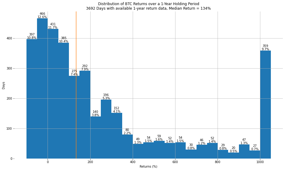
which_period = '1-year return'
plt.figure(figsize=(16,9), facecolor='white')
bins=np.arange(-100,1100,50)
plt.hist(np.clip(d[which_period], bins[0], bins[-1]),
         bins=bins)
plt.grid()
for spine in plt.gca().spines.values():
    spine.set_visible(False)
plt.ylabel('Days')
plt.xlabel('Returns (%)')
plt.title('''Distribution of BTC Returns over a 1-Year Holding Period
{} Days with available 1-year return data, Median Return = {}%'''
          .format(d[~d[which_period].isna()].shape[0],
                  int(round(d[which_period].median(),0))))
rects = plt.gca().patches
for n, r in enumerate(rects):
    height = r.get_height()
    plt.gca().text(r.get_x() + r.get_width() / 2,
                   height + 10,
                   (str(int(height)) + '\n'
                    + str(((height/d[~d[which_period].isna()].shape[0])*100.)
                          .round(1)) + '%'),
                   ha='center',
                   va='center')
plt.axvline(d[which_period].median(),
            c='C1');
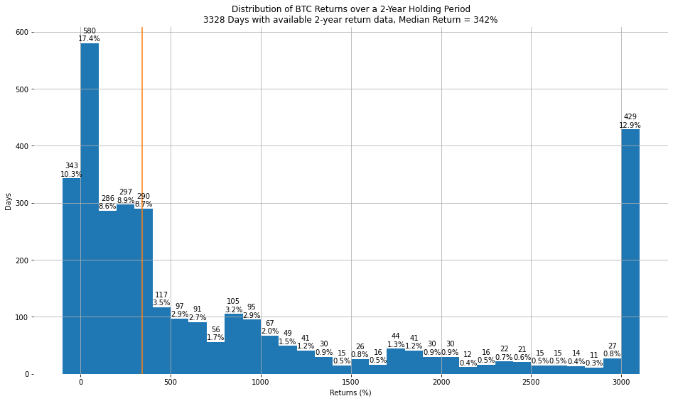
which_period = '2-year return'
plt.figure(figsize=(16,9), facecolor='white')
bins=np.arange(-100,3200,100)
plt.hist(np.clip(d[which_period], bins[0], bins[-1]),
         bins=bins)
plt.grid()
for spine in plt.gca().spines.values():
    spine.set_visible(False)
plt.ylabel('Days')
plt.xlabel('Returns (%)')
plt.title('''Distribution of BTC Returns over a 2-Year Holding Period
{} Days with available 2-year return data, Median Return = {}%'''
          .format(d[~d[which_period].isna()].shape[0],
                  int(round(d[which_period].median(),0))))
rects = plt.gca().patches
for n, r in enumerate(rects):
    height = r.get_height()
    plt.gca().text(r.get_x() + r.get_width() / 2,
                   height + 15,
                   (str(int(height)) + '\n'
                    + str(((height/d[~d[which_period].isna()].shape[0])*100.)
                          .round(1)) + '%'),
                   ha='center',
                   va='center')
plt.axvline(d[which_period].median(),
            c='C1');
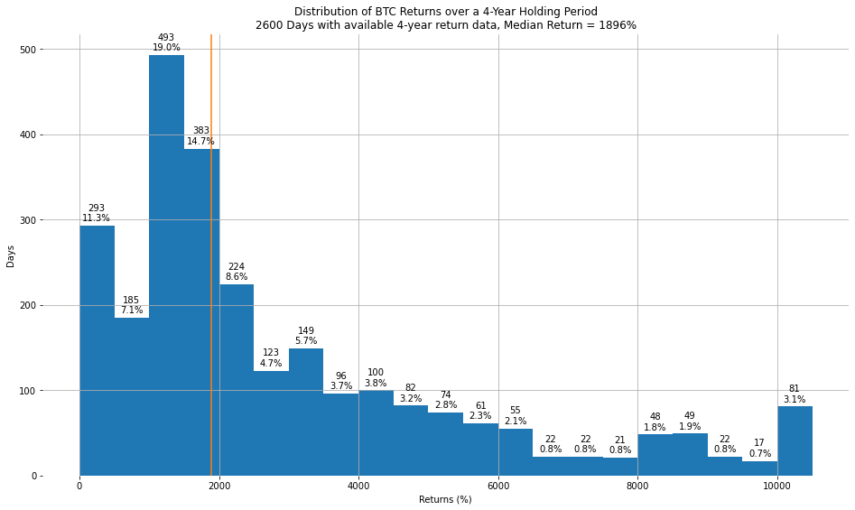
which_period = '4-year return'
plt.figure(figsize=(16,9), facecolor='white')
bins=np.arange(0,11000,500)
plt.hist(np.clip(d[which_period], bins[0], bins[-1]),
         bins=bins)
plt.grid()
for spine in plt.gca().spines.values():
    spine.set_visible(False)
plt.ylabel('Days')
plt.xlabel('Returns (%)')
plt.title('''Distribution of BTC Returns over a 4-Year Holding Period
{} Days with available 4-year return data, Median Return = {}%'''
          .format(d[~d[which_period].isna()].shape[0],
                  int(round(d[which_period].median(),0))))
rects = plt.gca().patches
for n, r in enumerate(rects):
    height = r.get_height()
    plt.gca().text(r.get_x() + r.get_width() / 2,
                   height + 15,
                   (str(int(height)) + '\n'
                    + str(((height/d[~d[which_period].isna()].shape[0])*100.)
                          .round(1)) + '%'),
                   ha='center',
                   va='center')
plt.axvline(d[which_period].median(),
            c='C1');