Suppor Vector Machines for Linear Classification

09 Feb 2020

Linear models can als be used for classification. This approach uses the same linear functional form as the more common form for regression, except we apply the sign function to the output of the linear function in order to produce a binary output that corresponds to the two possible class labels.

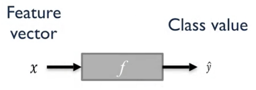$$f(x,w,b)=sign(w \cdot x + b)=sign(\sum w[i]x[i]+b)$$

The actual classification is computed using the equation of the separating line, in this case, $x_1 - x_2 = 0$. 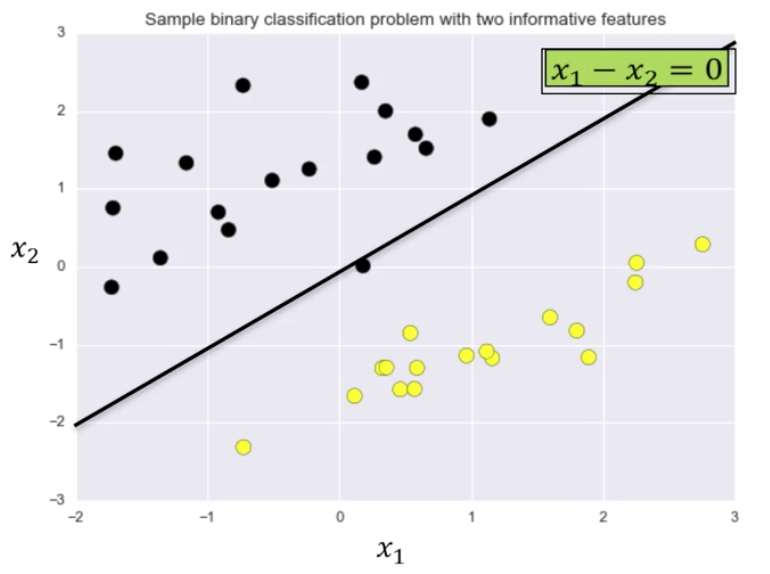The weights, $w$, and bias, $b$, are plugged into the formula along with the specific point being tested.

$$f(x, w, b)=sign(w \cdot x + b)$$

For the 2-D case,

$$f(x, w, b)=sign(w_1 x_1 + w_2 x_2 + b)$$

For this example, the point is $X = [-0.75, -2.25]$, $w = [1, -1]$, and $b=0$, so then:

$$f(x, w, b)=f([-0.75, -2.25],[1, -1],0)$$ $$=[sign((1 \cdot -0.75) + (-1 \cdot -2.25) + 0)$$ $$=sign(-0.75 + 2.25)$$ $$= sign(1.5) = +1$$

Classifier Margin

One way to to define a “good” classifier is by the amount of classifier margin they provide. Classifier margin is defined as the maximum width (or separation) the decision boundary area can be increased before hitting a data point. 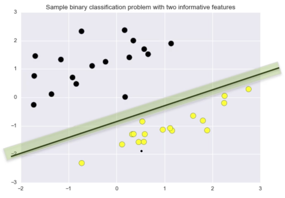The classifier the image below has a larger margin on this dataset than the classifier in the image above. 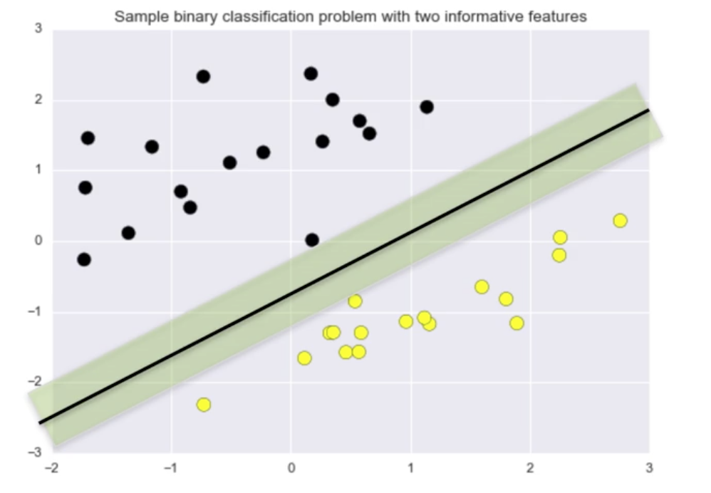The linear classifier with maximum margin is a Support Vector Machine, also known a Linear Support Vector Machine (LSVM), and as a Support Vector Machine with Linear Kernel.

SVMs in scikit-learn

Support Vector Machines operate similarly to the other classifier models in scikit-learn, using the fit method.

Synthetic Binary Classification Dataset

from sklearn.svm import SVC

X_train, X_test, y_train, y_test = train_test_split(X_C2, 
                                                    y_C2, 
                                                    random_state = 0)

fig, subaxes = plt.subplots(1, 1, figsize=(7, 5))

this_C = 1.0
clf = SVC(kernel = 'linear', 
          C=this_C)
clf.fit(X_train, y_train)
title = 'Linear SVC, C = {}'.format(int(this_C))
plot_class_regions_for_classifier_subplot(clf, 
                                          X_train, 
                                          y_train, 
                                          None, 
                                          None, 
                                          title, 
                                          subaxes)

<IPython.core.display.Javascript object>

The C parameter is used to control how tolerant the SVC is of misclassifications. C is a regularization parameter. It defaults to 1.0.

Larger values of C represent less regularization. It means the model will fit the training set with as few errors as possible, even if the classifier ends up with less overall margin. Smaller values of C use more regularization, and mean the classifier will find a large margine on the decision boundary, even if that decision boundary leads to more points being misclassified.

from sklearn.svm import LinearSVC

fig, subaxes = plt.subplots(1, 2, figsize=(8, 4))

for this_C, subplot in zip([0.00001, 100], subaxes):
    clf = LinearSVC(C=this_C,
                    max_iter=100000)
    clf.fit(X_train, y_train)
    title = 'Linear SVC, C = {:.5f}'.format(this_C)
    plot_class_regions_for_classifier_subplot(clf, 
                                              X_train, 
                                              y_train,
                                              None, 
                                              None, 
                                              title, 
                                              subplot)
plt.tight_layout()

<IPython.core.display.Javascript object>

Real-World Breast Cancer Dataset

The SVN performs very well, even without parameter tuning.

X_train, X_test, y_train, y_test = train_test_split(X_cancer, 
                                                    y_cancer, 
                                                    random_state = 0)

clf = LinearSVC(max_iter=100000).fit(X_train, y_train)
print('Breast cancer dataset')
print('Accuracy of Linear SVC classifier on training set: {:.2f}'
     .format(clf.score(X_train, y_train)))
print('Accuracy of Linear SVC classifier on test set: {:.2f}'
     .format(clf.score(X_test, y_test)))

Breast cancer dataset
Accuracy of Linear SVC classifier on training set: 0.91
Accuracy of Linear SVC classifier on test set: 0.92


/Users/ryanwingate/anaconda3/lib/python3.7/site-packages/sklearn/svm/_base.py:947: ConvergenceWarning: Liblinear failed to converge, increase the number of iterations.
  "the number of iterations.", ConvergenceWarning)

Linear Model - Advantages and Disadvantages

Note: Applicable to both linear and logistic regression.

Advantages

Simple and easy to train
Fast prediction
Scale well to very large datasets. SVMs use only a subset of the training points.
Works with sparse data
Results are easy to interpret

Disadvantages

Other models may generalize better on low-dimensional data
Data may not be linearly separable, but, SVNs can be trained with non-linear kernels as well

Functions Called Above

%matplotlib notebook

import numpy as np
import matplotlib.pyplot as plt
from matplotlib.colors import ListedColormap
from sklearn.datasets import make_classification
from sklearn.model_selection import train_test_split
from sklearn.svm import SVC

Real-world breast cancer dataset

from sklearn.datasets import load_breast_cancer

(X_cancer, y_cancer) = load_breast_cancer(return_X_y = True)

Synthetic binary classification dataset

X_C2, y_C2 = make_classification(n_samples = 100, n_features=2,
                                 n_redundant=0, n_informative=2,
                                 n_clusters_per_class=1, flip_y = 0.1,
                                 class_sep = 0.5, random_state=0)

def plot_class_regions_for_classifier_subplot(clf, X, y, X_test, y_test, title, subplot, 
                                              target_names = None, 
                                              plot_decision_regions = True):

    numClasses = np.amax(y) + 1
    color_list_light = ['#FFFFAA', '#EFEFEF', '#AAFFAA', '#AAAAFF']
    color_list_bold = ['#EEEE00', '#000000', '#00CC00', '#0000CC']
    cmap_light = ListedColormap(color_list_light[0:numClasses])
    cmap_bold  = ListedColormap(color_list_bold[0:numClasses])

    h = 0.03
    k = 0.5
    x_plot_adjust = 0.1
    y_plot_adjust = 0.1
    plot_symbol_size = 50

    x_min = X[:, 0].min()
    x_max = X[:, 0].max()
    y_min = X[:, 1].min()
    y_max = X[:, 1].max()
    x2, y2 = np.meshgrid(np.arange(x_min-k, x_max+k, h), 
                            np.arange(y_min-k, y_max+k, h))

    P = clf.predict(np.c_[x2.ravel(), y2.ravel()])
    P = P.reshape(x2.shape)

    if plot_decision_regions:
        subplot.contourf(x2, 
                         y2, 
                         P, 
                         cmap=cmap_light, 
                         alpha = 0.8)

    subplot.scatter(X[:, 0], 
                    X[:, 1], 
                    c=y, 
                    cmap=cmap_bold, 
                    s=plot_symbol_size, 
                    edgecolor = 'black')
    subplot.set_xlim(x_min - x_plot_adjust, 
                     x_max + x_plot_adjust)
    subplot.set_ylim(y_min - y_plot_adjust, 
                     y_max + y_plot_adjust)

    if (X_test is not None):
        subplot.scatter(X_test[:, 0], 
                        X_test[:, 1], 
                        c=y_test, 
                        cmap=cmap_bold, 
                        s=plot_symbol_size, 
                        marker='^', edgecolor = 'black')
        train_score = clf.score(X, y)
        test_score  = clf.score(X_test, 
                                y_test)
        title += "\nTrain score = {:.2f}, Test score = {:.2f}".format(train_score, 
                                                                      test_score)

    subplot.set_title(title)

    if (target_names is not None):
        legend_handles = []
        for i in range(0, len(target_names)):
            patch = mpatches.Patch(color=color_list_bold[i], 
                                   label=target_names[i])
            legend_handles.append(patch)
        subplot.legend(loc=0, handles=legend_handles)

These notes were taken from the Coursera course Applied Machine Learning in Python. The information is presented by Kevyn Collins-Thompson, PhD, an associate professor of Information and Computer Science at the University of Michigan.