Neural Networks
An artificial neural network is analogous to the network of biological neurons that comprise our brains.
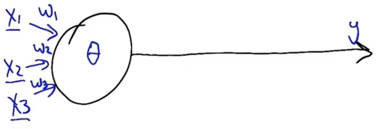
Perceptron
The inputs to each perceptron unit are at least one signal, $x_i$. These signals are multiplied by a weight, $w_i$ which amplifies or attenuates the signal depending on its magnitude.
For each perceptron unit, the input and weights are multiplied and summed to determine the neuron’s activation. If the activation is greater than the neuron’s firing threshold, $\theta$, then the neuron’s output is 1, otherwise it is 0.
$$Activation = \sum_{i=1}^{k} x_i w_i$$ $$Activation \geq \theta, \rightarrow output = 1$$ $$Activation < \theta, \rightarrow output = 0$$
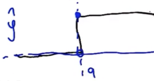
For $w_1=\frac{1}{2}$, $w_2=\frac{1}{2}$, $\theta=\frac{3}{4}$, the output space of the single neuron follows. Green indicates an output of 1, red indicates an output of 0.
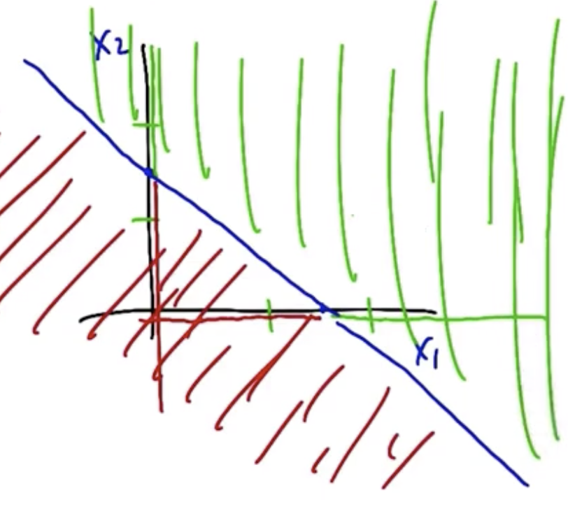
Perceptrons compute halfplanes, the right side of which indicates an output of 1, the left side of which indicates an output of 0.
Function Examples
For $w_1=\frac{1}{2}$, $w_2=\frac{1}{2}$, $\theta=\frac{3}{4}$ and $x_1 \in (0,1)$, $x_2 \in (0,1)$, y computes the AND function.
For $w_1=\frac{1}{2}$, $w_2=\frac{1}{2}$, $\theta=\frac{1}{4}$ and $x_1 \in (0,1)$, $x_2 \in (0,1)$, y computes the OR function.
For $w_1=-1$, $\theta=0$ and $x_1 \in (0,1)$, y computes the NOT function.
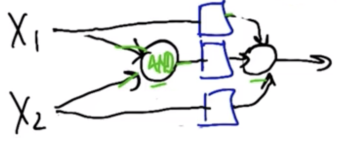
XOR can be modeled by the following two-perceptron unit structure, if weights of $1$, $-2$, and $1$ are assigned top-to-bottom.
Perceptron Training
There are two mechanisms by which Perceptron weights can be computed from examples:
- Perceptron rule (includes thresholds)
- Gradient descent/delta rule (does not include threshold)
Perceptron Rule
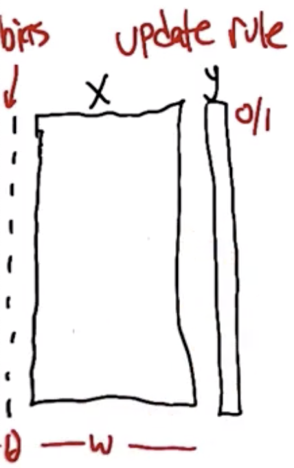
The perceptron rule is how to set the weights of a single unit such that it matches some training set. We assume the existence of training set of vectors, $x$, and corresponding outputs $y$. Subtract the activation energy, $\theta$, from both sides of the activation function $\hat{y} = \sum_{i} w_i x_i \geq \theta$, such that it essentially becomes its own weight which is learned along with the other weights. This simplifies the mathematics. A bias term of a constant 1 to accommodate this, and the weight that corresponds to that bias is $\theta$.
The algorithm is while there is some error, iterate over:
$$w_i = w_i + \Delta w_i$$
$$\Delta w_i = \eta (y - \hat{y}) x_i$$
$$\hat{y} = \sum_{i} w_i x_i \geq 0$$
where $y$: target, $\hat{y}$: output, $\eta$: learning rate, and $x$: input.
| $y$ | $\hat{y}$ | $y - \hat{y}$ |
|---|---|---|
| 0 | 0 | 0 |
| 0 | 1 | -1 |
| 1 | 0 | 1 |
| 1 | 1 | 0 |
If there is a half-plane that can cleanly separate the data, then the dataset is called linearly separable, as shown below.
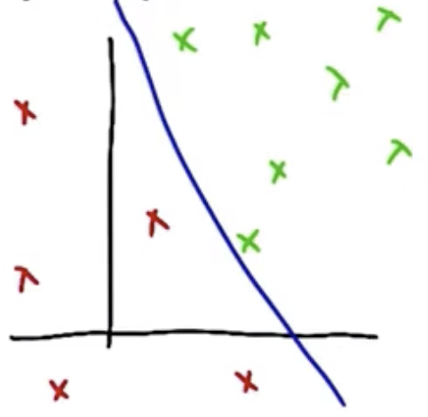
If the dataset is linearly separable, then the perceptron rule will find the half-plane that separates it with finite iterations. For high-dimensional datasets, it is generally not possible to know ahead of time whether the dataset is linearly separable, however, so a algorithm that is more robust to non-linearly-separable data is generally required.
Gradient Descent
Gradient Descent is very analogous to the Perceptron Rule.
Define an “activation”, $a$, as follows:
$$a = \sum_{i} x_i w_i$$
The esimated output, $\hat{y}$, is whether or not that activation is greater than 0, because we assume the output is not thresholded.
$$\hat{y} = (a \geq 0 )$$
Then, we define an error metric on the weight vector w, $E(w)$, as follows:
$$E(w) = \frac{1}{2}\sum_{(x,y)\in D} (y-a)^2$$
The goal in gradient descent is to minimize the quantity shown above. Using Calculus, take the partial derivative of the error metric with respect to the weights. The idea is that we are looking for the direction to push the weights which will cause the error to decrease.
$$\frac{\partial{E}}{\partial{w_i}} = \frac{\partial}{\partial{w_i}} \frac{1}{2} \sum_{(x,y)\in D} (y-a)^2$$
Using the chain rule with $a = \sum_{i} x_i w_i$:
$$\frac{\partial{E}}{\partial{w_i}} = \sum_{(x,y)\in D} (y-a)(-x_i)$$
Comparison of Perceptron versus Gradient Descent Learning Rules
Perceptron update rule:
$$\Delta w_i = \eta(y-y_i)x_i$$
- Guaranteed convergence for linearly separable data
Gradient Descent update rule:
$$\Delta w_i = \eta(y-a)x_i$$
- Robust to datasets that are not linearly-separable
- Converges to a local optimum
Question arises, why not do gradient descent on $\hat{y}$? Because it is non-differentiable.
Therefore, convert the activation function to a sigmoid, which resembles the step change shown above but which is differentiable. So, use the sigmoid function:
$$\sigma (a) = \frac{1}{1 + e^{-a}}$$
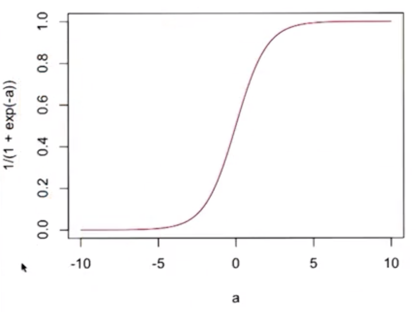
$$D\sigma(a) = \sigma(a)(1-\sigma(a))$$
- The derivative of the sigmoid function (shown above) has a simple form.
- It also goes to 0 as activation gets small, and
- it goes to 1 as the activation gets large.
For those reasons, it is ideal for this use case, but there are other functions that would work as well.
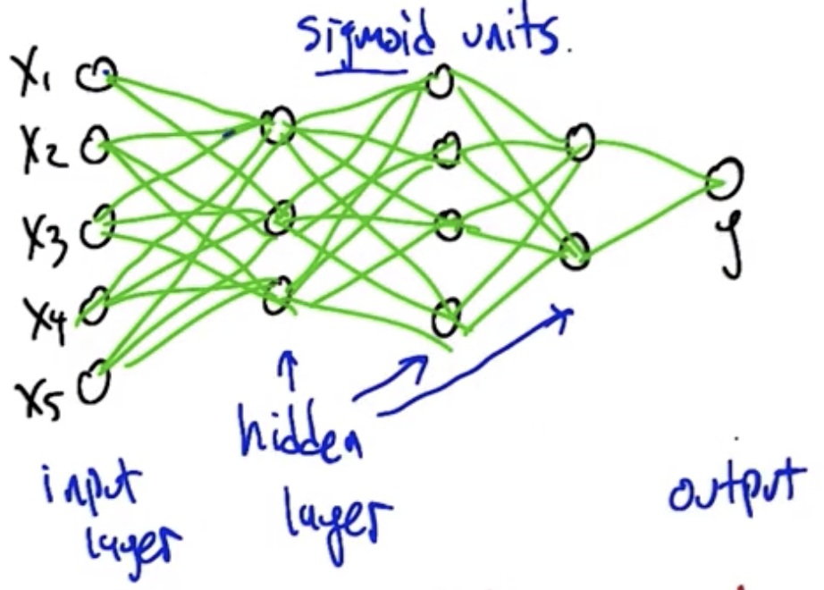
Networks of Neurons
By using the sigmoid function as the activation function, it becomes possible to create large networks of sigmoid units, as shown below. Crucially, the entire structure is differentiable. So, it becomes possible to calculate the impact of changing any given weight in the structure on the overall mapping from input to output.
Backpropagation: a computationally beneficial organization of the chain rule, wherein information flows from the inputs to the outputs, and error information flows backward from the outputs toward the inputs. This information allows you to compute all of the derivatives, and therefore how to make all of the weight changes so the structure converges on the correct set of outputs.
These structures are analogous to a perceptron but not identical to a perceptron. In particular, there is no guarantee that the structure will converge onto a solution as with the perceptron. These strucutres can have many local optima, wherein it becomes impossible for any of the weights to change without increasing the overall error of the system. The “error surface” is a parabola in a high-dimensional space that is smooth, but which has many local minima that are not necessarily the global minimum.
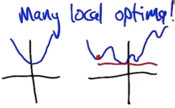
There are many advanced optimization methods that enable avoiding these local optima:
- Momentum terms in the gradient
- Higher order derivatives
- Randomized optimizations
- Penalty for “Complexity”
Neural networks increase in complexity through:
- Adding more nodes,
- Adding more layers, and having
- larger weights.
Restriction Bias
Recall restriction bias relates to the representational power of the data structure being employed. It is the set of hypotheses that are under consideration.
Perceptrons: restricted to modeling half-spaces (like lines, in 2D).
Sigmoids: much more complex, not much restriction
Using a sufficiently-complex networks of threshold-like units, it is possible to model:
- Any Boolean function,
- Any Continuous (IE, connected, no jumps) function can be modeled with a single hidden layer.
- Any Arbitrary (IE, any input-to-output mapping even discontinuous) function can be modeled with two hidden layers.
So, neural networks are not very restrictive at all. This means that when using neural networks there is increased danger of overfitting. Overfitting can be eliminated by imposing limits on the number of hidden units and layers. Using neural networks in general doesn’t have much restriction bias, but a specific neural network architecture does have limitations.
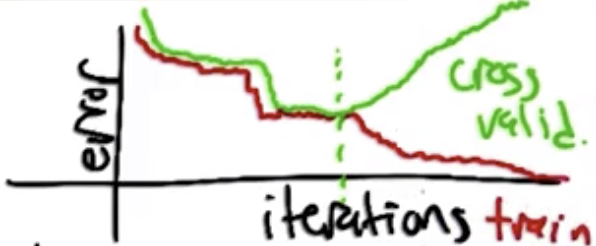
As with regression, cross validation can be used to help determine how many layers, hidden units, and scale of the weights to use. When cross validation error begins increasing, typically it indicates some of the weights are growing large.
Initial Weights
The initial weights that are typically used are small random values, for two reasons:
- Helps to avoid local minima, and
- Variability - it ensures that if the algorithm is run multiple times it doesn’t stuck in the same place.
Preference Bias
Recall preference bias pertains to the solution set the algorithm being employed converges to.
- Prefers low “complexity”
- Prefers simpler explanations, provided the correct algorithm is employed:
- Weights start with small random values, and
- Algorithm stops once you start overfitting.
Reminiscient of Occam’s Razor: “Entities should not be multiplied unnecessarily,” where:
- “unecessarily”, in the case of neural networks, means that additional training does not help improve the fit to the data, and
- “multiplied” means make more complex.
For Fall 2019, CS 7461 is instructed by Dr. Charles Isbell. The course content was originally created by Dr. Charles Isbell and Dr. Michael Littman.