Instance Based Learning
Instance Based Learning distinguishes itself from techniques like Decision Trees, Neural Networks, and Regression in one key way. Those techniques implicitly involved discarding the inputs/training data. Specifically, future predictions made by those artifacts did not require explicitly referencing the input data.
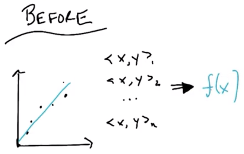
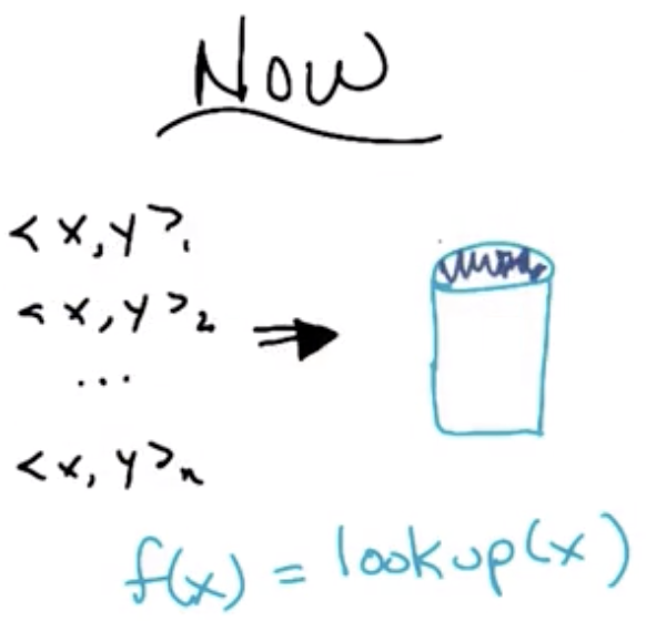
In the Instance Based Learning paradigm, the training data is explicitly stored in a database instead and referenced for future predictions.
Positive aspects:
- highly reliable: actual data is explicitly stored and remembered,
- fast: it only involves database writes and reads, and
- simple: no interesting learning takes place.
Negative aspects:
- No generalization: data are stored explicitly,
- Possible to overfit: due to “bottling the noise,” exactly
- Duplicate values likely to cause a problem.
Worked Example
In the following image:
Red represents expensive homes, Blue represents moderately-expensive homes, and Green represents inexpensive homes.
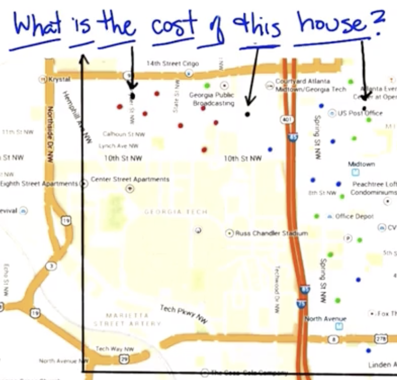
Using a nearest neighbor approach, we infer that the value of the black dots are the same as the nearest labeled dot.
A logical extension of that approach would be a k nearest neighbors approach, which could involve taking the value of the five nearest neighbors (for example) and computing an average. This approach would have two free parameters:
- K, the number of neighbors, and
- similarity, which could be distance, in the case of a map, but could also include other features like number of bedrooms, school district, square footage, etc.
K Nearest Neighbor Algorithm
Given:
- Training data: $D={x_i, y_i}$
- Distance metric: $d(q,x)$, which represents our domain knowledge
- Number of Neighbors: $k$, also domain knowledge
- Query Point: $q$
Find:
- Set of nearest neighbors, NN
$$NN = ${i: d(q,x_i)\ k\ smallest}$$
Return:
- Classification: possibly weighted, plurality vote of the $y_i \in NN$
- Regression: possibly weighted, mean of the $y_i \in NN$
Note that the complexity of this algorithm is mostly in the design of the distance metric, choice of $k$, methods for breaking tie votes, etc.
Algorithm Big O Comparison
Running Time: time required to accomplish the task Space: space in memory required to accomplish the task
Given $n$ sorted data points, the Big O running time and space classifications are shown below.
| Learning Algorithm | Operation Type | Running Time | Space |
|---|---|---|---|
| 1 Nearest Neighbor | Learning | 1 | $n$ |
| Query | $\log n$ | 1 | |
| K Nearest Neighbor | Learning | 1 | $n$ |
| Query | $\log n + k$ | $1$ | |
| Linear Regression | Learning | $n$ | 1 |
| Query | 1 | 1 |
Given the Big O classifcations above, Nearest Neighbor approaches are usually referred to as lazy learners, as they postpone doing any “learning” until absolutely necessary, specifically at query time. Linear regression, on the other hand, is an eager learner, because it performs the “learning,” in the form of calculating the regression, during training.
Worked Prediction Using K-NN
Given the following query point and the $\mathbb{R}^2 \rightarrow \mathbb{R}$ mapping shown below, compute the outputs below, where $d()$ indicates the distance metric being employed.
$$q=(4,2)$$
| X | Y | $Manhattan$ | $Euclidean^2$ |
|---|---|---|---|
| (1,6) | 7 | 7 | 25 |
| (2,4) | 8 | 4 | 8 |
| (3,7) | 16 | 6 | 24 |
| (6,8) | 44 | 8 | 40 |
| (7,1) | 50 | 4 | 10 |
| (8,4) | 68 | 6 | 20 |
| d() | K | Average |
|---|---|---|
| Euclidean | 1-NN | 8 |
| 3-NN | 42 | |
| Manhattan | 1-NN | 29 |
| 3-NN | 35.5 |
The function used to calculate $y$ was $y=x_1^2 + x_2$, so the “actual” output for $q=(4,2)$ was $4^2+2=18$.
Preference Bias
Recall Preference Bias is our notion of why the algorithm being employed would prefer one hypothesis over another, all other things being equal. It is the thing that encompasses a given algorithms' “belief” about what makes a good hypothesis. Every algorithm has preference biases built in.
- Locality: Near points are similar by definition.
- The specific distance function being employed also involves implicit assumptions about what constitutes “near” points.
- For any given fixed problem, there is some ideal distance function that minimizes errors versus other functions, but finding it may be arbitrarily difficult.
- Smoothness
- Choosing to average near points, the assumption is that functions will behave smoothly, without large jumps.
- All features matter equally
Curse of Dimensionality
The following is a fundamental theorem or “result” of machine learning that is particularly relevant to K-NN, but is applicable to all of maching learning.
- As the number of features or dimensions grows, the amount of data we need to generalize accurately grows exponentially!
- Number of features/dimensions given by $n$ in $x_1,\ x_2,\ …\ x_n$.
- What this implies, practically, is that simply adding features to an input space will not necessarily make a given algorithm perform better.
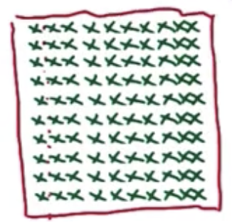
To visualize this, imagine the following 10 datapoints exist in a 1-dimensional space. Each represents 10% of the line segment.

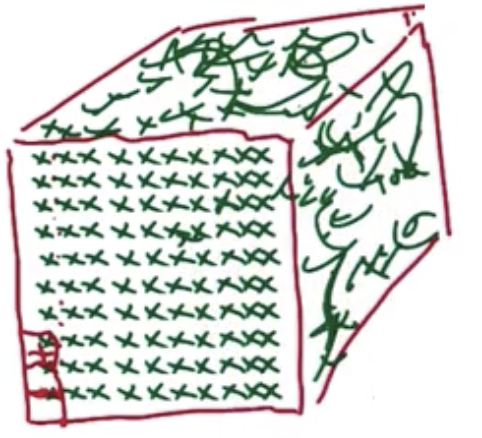
Now image a similar ten datapoints in a 2-dimensional space. Each still represents 10% of the total space.
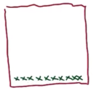
In order to occupy the space more completely, it is necessary to have much more data.
This scales to higher dimensions as well.
So, to cover a higher-dimensional input space, something on the order of $10^d$ datapoints would be required, where $d$ is the number of dimensions. So, to improve performance of a machine learning algorithm, it is better to give more data than to give more dimensions. Future lessons will discuss means of finding the right dimensionality for ML problems.
Other Items
- Distance function choice matters! $d(x,q)$
- Some options: Euclidean (weighted, unweighted), Manhattan (weighted, unweighted)
- Other examples could involve more computationally complex ideas of distance, particularly for images, that might involve items like distance between eyes, size of mouth, etc.
- For K Nearest Neighbors with $K\ \rightarrow\ n$ (“K approaching n”), we can:
- perform a weighted average wherein points near the query point, $q$ are granted more weight/importance, or
- perform a locally weighted regression using the original points, or use something even more general (decision tree, neural network, lines, etc)
- Practically, this means that though we begin with a hypothesis space of lines, we end up with a more complex hypothesis space that can include curves.
- “Instance” Based Learning is so-called because it involves looking at very specific instances and using that subset to inform the learning that takes place.
For Fall 2019, CS 7461 is instructed by Dr. Charles Isbell. The course content was originally created by Dr. Charles Isbell and Dr. Michael Littman.