Computational Learning Theory
Computational Learning Theory gives us a formal way of addressing three important questions:
- Definition of a learning problem,
- Showing specific algorithms work, and
- Show some problems are fundamentally hard (or unsolvable).
- The tools and analyses that are used in learning theory are the same tools and analyses that are used in computing:
- Theory of computing analyzes how algorithms use resources like time and space, specifically, algorithms may be $O(n \log n)$ or $O(n^2)$, for example.
- In computational learning theory, algorithms use time, space, and samples (or data, examples, etc.)
Defining Inductive Learning
- Probability of successful training:
- $1-\delta$
- Number of examples to train on:
- $m$
- Complexity of hypothesis class, or,
- complexity of $H$
- Accuracy to which target concept is approximated:
- $\epsilon$
- Manner in which training examples are presented:
- batch / online
- Manner in which training examples are selected:
- Learner asks questions of teacher
- c(x) = ?
- Teacher gives examples to help learner
- Teacher chooses x, tells c(x)
- Fixed distribution
- $x$ chosen from $D$ by nature
- Worst possible distribution
- Learner asks questions of teacher
20 Questions Example
Consider the teaching via 20 Questions example
where:
- $H$: set of possible answers
- $X$: set of questions
- Assume the teacher knows the answer, but the learner does not
If the teacher chooses the question, $X$, then it may take as few as $1$ questions to determine the answer.
If the learner chooses the question, $X$, then it will take $\log_2 |H|$ questions to determine the answer.
Teacher with Constrained Queries
x: $x_1, x_2, …, x_k$, k-bit inputs
h: conjunctions of literals or negation, for example:
$h: x_1\ and\ x_3\ and\ \overline{x_5}$
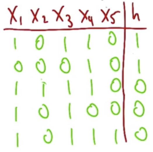
In the following examples, the $H$ are given as outputs of this expression.
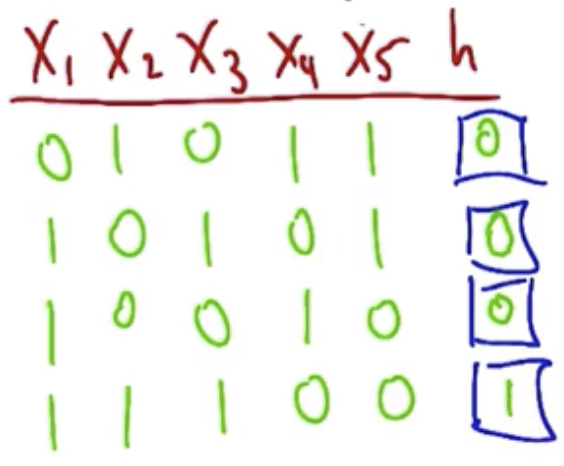
It is also possible to pose questions about moving in the other direction. For example, given these outputs, what is the exact hypothesis?
Approaching this requires a two-stage process:
- Show which parameters are irrelevant (in the example above, $x_1$ and $x_3$ were irrelevant, because they were inconsistent despite a consistent output).
- Show which parameters are relevant (in the example above, $x_2$, $x_4$, and $x_5$ are all relevant).
The specific hypothesis is:
$\overline{x_2}\ and\ x_4\ and\ \overline{x_5}$
There are $3^k$ possible hypotheses, which could be learned with $k \log_2 {3}$, which is linear in $k$.
Learner with Constrained Queries
In the example of a learner that does not have a teacher to choose questions to help teach it the hypothesis, it becomes necessary for the learner to ask all possible data points before finding a hypothesis that outputs 1. In particular, it could take as many as $2^k$ queries.
Learner with Mistake Bands
The mistake bands learning formalism involves the following loop:
- Input arrives,
- Learner guesses answer,
- If wrong answer, add to a mistake counter,
- Repeat.
The total number of mistakes is limited to some value.
A more precise algorithm would involve:
- Assume each variable $X$ is present in the hypothesis in both its positive and negative forms (IE, $x_1\ and\ \overline{x_1}\ and\ …$),
- Given input, compute output,
- If wrong, set all positive variables that were 0 to “absent,” negative variables that were 1 to absent.
- Go to step 2.
In this schema, the learner would never make more than $K+1$ mistakes.
Definitions
Computational Complexity: How much computational effort is needed for a learner to converge
Sample Complexity (batch): How many training examples are needed for a teacher to create a successful hypothesis
Mistake bounds (online): How many misclassifications can a learner make over an infinite run
Recall that there are three ways of choosing the inputs to the learner: learner chooses, teacher chooses, nature chooses, and worst possible distribution. The nature chooses way of learning will be considered next. It is unique in that it requires you to take into account the space of possible distributions.
Hypothesis space: $H$,
True hypothesis: $c \in H$, also called a concept
Training set: $S \subseteq X$, a subset of the possible inputs, along with $c(x)\ \forall\ x \in S$
Candidate hypothesis: $h \in H$
Consistent learner: produces $c(x)=h(x)$ for $x \in S$, a consistent learners is able to learn the true hypothesis. It is called consistent because it is consistent with the data.
Version space: $VS(S)$ = $\lbrace h \ |\ h\ \in\ H\ consistent\ with\ S\rbrace$, IE, “the version space for a given set of data, $S$, is the set of hypotheses that are in the hypothesis set such that they are consistent with respect $S$”
Version Space Example
An example target concept is shown below. It is the $XOR$ function.
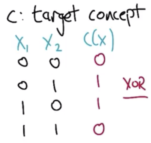
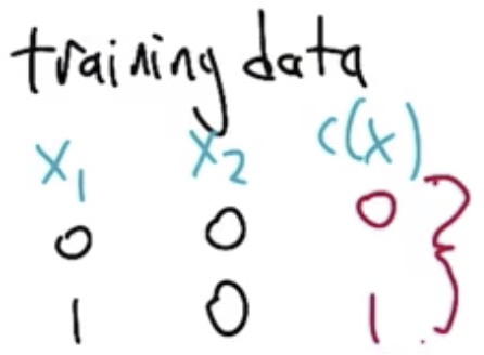
The training data, $S$ is shown below.
The hypothesis set, $H$, is given below.
$H = \lbrace x_1, \overline{x_1}, x_2, \overline{x_2}, T, F, OR, AND, XOR, EQUIV \rbrace $
Which elements in $H$ are in the version space, $VS$?
$VS = \lbrace x_1, OR, XOR \rbrace$
PAC Learning
Training Error: fraction of training examples misclassified by h.
True Error: fraction of examples that would be misclassified on sample drawn from D.
The error of h is defined as follows. This formula captures the notion that it is okay to misclassify examples that will be seen rarely see. The penalty is in proportion to the probability of getting it wrong.
$$error_{D}(h)= Pr_{x \sim D} [c(x) \neq h(x)]$$
PAC stands for Probably Approximately Correct, where probably is a stand-in for $1-\delta$, approximately is a stand-in for $\epsilon$, and correct is a stand-in for $error_D(h)=0$
$C$: concept class
$L$: learner
$H$: hypothesis space
$n$: $|H|$, size of hypothesis space
$D$: distribtion over inputs
$0 \leq \epsilon \leq \frac{1}{2}$: Error Goal, error should be less than $\epsilon$
$0 \leq \delta \leq \frac{1}{2}$: Certainty Goal, certainty is ($1-\delta$)
PAC-learnable: a concept, $C$, is PAC-learnable by $L$ using $H$ if and only if learner, $L$ will, with probability $(1-\delta)$, output a hypothesis $h \in H$ such that $error_D(h)\leq \epsilon$ in time and samples polynomial in $\lbrace \frac{1}{\epsilon}, \frac{1}{\delta}, n \rbrace$
$\epsilon$-exhausted version space: $VS(S)$ is $\epsilon$-exhausted iff $\forall\ h \in\ VS(S)$ $error_D(h) \leq \epsilon$. In other words, a version space is called $\epsilon$-exhausted exactly in the case when everything that might be chosen has an error less than $\epsilon$.
$\epsilon$-exhausted Version Space Example
Given the following training set and associated distributions, find the smallest $\epsilon$ such that we have $\epsilon$-exhausted the version space.
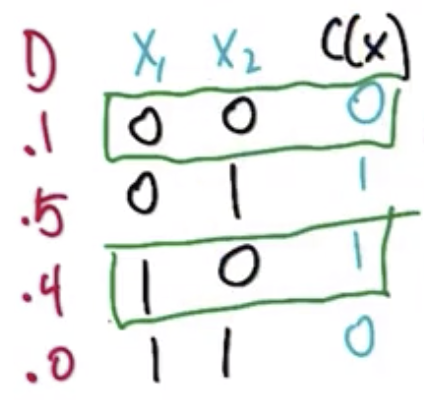
The hypothesis space is $H = \lbrace x_1, \overline{x_1}, x_2, \overline{x_2}, T, F, OR, AND, XOR, EQUIV \rbrace$. The target concept is $XOR$ and the training set are the inputs in the green boxes. The distribution, $D$, gives the probability of drawing each of these input examples. Recall from the previous question that the version space is $VS = \lbrace x_1, OR,XOR\rbrace$
| Version Space | True Error |
|---|---|
| $x_1$ | 0.5 |
| $OR$ | 0.0 |
| $XOR$ | 0.0 |
The input $x_1$ has a true error of 0.5 because half the time it will be presented with the second training set, which it will get incorrect. Both $OR$ and $XOR$ will not give an error. So, the minimum $\epsilon$ over which the version space is exhausted is the max true error for the $VS$, or 0.5.
Haussler Theorem - Bound True Error
Let $error_D (h_1,…,h_k\in H) \geq \epsilon$. These hypotheses have “high true error.” How much data do we need to establish that these hypotheses are “high error?”
The following formula says that the probability that if you draw an input, $x$ from the distribution, $D$, the “bad” hypotheses will match the true concept is less than or equal to $1-\epsilon$. IE, there is a low probability of match.
$$Pr_{X \sim D} (h_i(x)=c(x)) \leq 1 - \epsilon$$
$$Pr (h_i\ remains\ consistent\ with\ c\ on\ m\ examples) \leq (1-\epsilon)^m$$
$$Pr (at\ least\ one\ of\ h_1,\ …,\ h_k\ consistent\ with\ c\ on\ m\ examples)$$
$$\leq k(1-\epsilon)^m \leq |H|(1-\epsilon)^m$$
Using the fact that $-\epsilon \geq len(1-\epsilon)$ we get $(1-\epsilon)^m \leq e^{-\epsilon m}$. Then $|H|(1-\epsilon)^m$ can be rewritten as
$$\leq |H|e^{-\epsilon m} \leq \delta$$
This is an upper bound that version space not $epsilon$-exhausted after $m$ samples. Recall that $\delta$ is a failure probability. Rewriting this in terms of m:
$$\ln|H|-\epsilon m \leq \ln \delta$$
$$m \geq \frac{1}{\epsilon}(ln|H| + ln \frac{1}{\delta})$$
This is called the sample complexity bound and it is important in that it depends polynomially on the target error ($\epsilon$) bound, the size of the hypothesis space ($|H|$), and the failure probability ($\delta$).
PAC-Learnable Example
$$H = \lbrace h_i(x) = x_i \rbrace,\ where\ x\ is\ 10\ bits$$
So, the hypothesis space is the set of functions that take 10 bit inputs and return each of those 10 bits. IE, one returns the first bit, one returns the second, etc.
$$\epsilon=0.1, \delta=0.2,\ D\ is\ uniform$$
That is to say that we want to return a hypothesis whose error is 0.1, and we want the failure probability to be less than 0.2, and the input distribution is uniform. How many samples do we need to PAC learn this hypothesis set?
$$m \geq \frac{1}{.1}(ln 10 + ln \frac{1}{.2}) \geq 39.12\ or\ 40\ samples$$
Note that this calculation is agnostic to the nature of the distribution.
Final Notes and Limitations
- If the target concept is not in the hypothesis space, the learning scenario is called “agnostic,” and the formula for the sample bound must be calculated differently. Generally speaking, in this scenario, more samples are required.
- If the size of the hypothesis space, $|H|$, is infinite, then the formula for the sample bound breaks down. This scenario will be discussed in a separate lecture.
These notes are continued in my notes on VC Dimensions.
For Fall 2019, CS 7461 is instructed by Dr. Charles Isbell. The course content was originally created by Dr. Charles Isbell and Dr. Michael Littman.