Bayesian Inference
Joint Distribution
The following is an example of a joint distribution.
| Storm | Lightning | Probability |
|---|---|---|
| T | T | .25 |
| T | F | .40 |
| F | T | .05 |
| F | F | .30 |
A few possible calculations:
$$Pr(\overline{Storm})=.30+.05=.35$$
$$Pr(Lightning|Storm)=.25/.65=.4615$$
Each additional category multiplies the space by the number of possible values of that category. For example, adding thunder would increase the space to 8 different categories.
Normal Independence
Independence means that the joint distribution of two variables is equal to the product of their marginals.
$$Pr(X,Y)=Pr(X)Pr(Y)$$
Chain Rule
$$Pr(X,Y)=Pr(X|Y)Pr(Y)$$
Substituting the first equation into the second, we get
$$\forall_{x,y} Pr(X|Y)=Pr(X)$$
Conditional Independence
$X$ is conditionally independent of $Y$ given $Z$ if the probability distribution governing $X$ is independent of the value of $Y$ given the value of $Z$; that is if
$$\forall_{x,y,z} P(X=x|Y=y, Z=z)=P(X=x|Z=z)$$
More compactly, this can be written:
$$P(X|Y,Z)=P(X|Z)$$
Conditional Independence Example
| Storm | Lightning | Thunder | Probability |
|---|---|---|---|
| T | T | T | .20 |
| T | T | F | .05 |
| T | F | T | .04 |
| T | F | F | .36 |
| F | T | T | .04 |
| F | T | F | .01 |
| F | F | T | .03 |
| F | F | F | .27 |
$$P(thunder=T|lightning=F,storm=T)=.04/.40=.10$$
$$P(thunder=T|lightning=F,storm=F)=.03/.30=.10$$
$$Pr(T|L,S)=Pr(T|L)$$
So, we have conditionally independent variables. Thunder is conditionally independent of Storm, given Lightning.
Bayesian Networks
Bayesian Networks, also known as Bayes Nets, Belief Networks, and Graphical Models, are graphical representations for the conditional independence relationships between all the variables in the joint distribution. Nodes correspond to variables and edges correspond to dependencies that need to be explicitly represented.
We have shown that Thunder is conditional independent of storm given lightning, so $P(Th|L,S)$ and $P(Th|L,\overline{S})$ and their variations are excluded. So, with the five numbers shown it is possible to work out any probability we want in the joint.
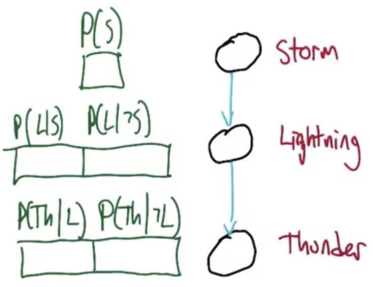
| Label | Probability |
|---|---|
| $P(S)$ | .650 |
| $P(L|S)$ | .385 |
| $P(L|\overline{S})$ | .143 |
| $P(Th|L)$ | .800 |
| $P(Th|\overline{L})$ | .100 |
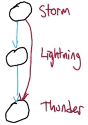
If Thunder were not conditionally independent of Storm given Lightning the network would be more complex. The number of values that need to be tracked grows exponentially with indegree of a given node.
Sampling from the Joint Distribution
The only appropriate order is topological, due to the dependencies. $A\sim P(A),\ B\sim P(B),\ C\sim P(C|A,B),\ D\sim P(D|B,C),\ E\sim P(E|C,D)$
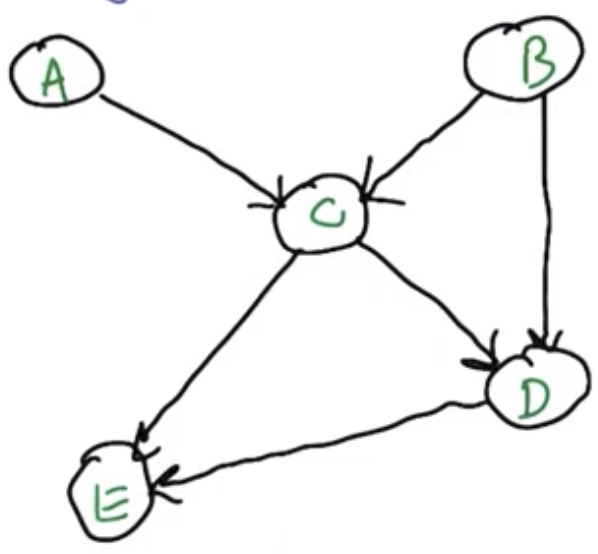
The network must always be directed and acyclic.
$$Pr(A,B,C,D,E)=Pr(A) Pr(B) Pr(C|A,B) Pr(D|B,C) Pr(E|C,D)$$
Why Sampling?
- Two things distributions are for:
- Determine probability of value
- Generate values
- Simulation of a complex process
- Approximate inference
- Visualization - get a feel for how the distribution works
Inferencing Rules
The following rules are often used in combination to work out the probabilities for various kinds of events.
Marginalization
$$P(x)=\sum_y P(x,y)$$
Chain Rule
$$P(x,y) = P(x)P(y|x)$$
Bayes Rule
$$P(y|x)=\frac{P(x|y)P(y)}{P(x)}$$
Marbles and Boxes Example
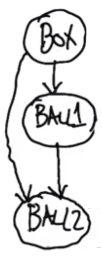
Consider example where someone picks a box, picks a ball from that box, then picks another ball from the same box without replacing the first ball.
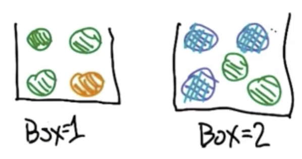
What is the probability of pulling out a green ball followed by a blue ball? $P(2=blue|1=green)$
The Baye’s net for this problem is.
Ball 1 Probabilities
| Box | Green | Yellow | Blue |
|---|---|---|---|
| 1 | 3/4 | 1/4 | 0 |
| 2 | 2/5 | 0 | 3/5 |
Ball 2 Probabilities, assuming ball 1 was green
| Box | Green | Yellow | Blue |
|---|---|---|---|
| 1 | 2/3 | 1/3 | 0 |
| 2 | 1/4 | 0 | 3/4 |
The formula below follows from the marginalization rule and the chain rule:
$$P(2=blue|1=green)=P(2=blue|1=green,box=1)P(box=1|1=green)$$ $$+P(2=blue|1=green,box=2)P(box=2|1=green)$$
The formulae below follows from Baye’s rule:
$$P(box=1|1=green)=P(1=green|box=1)\frac{Pr(box=1)}{Pr(1=green)}$$
$$P(box=2|1=green)=P(1=green|box=2)\frac{Pr(box=2)}{Pr(1=green)}$$
The following comes from averaging the likelihood of the first draw being a green, given that the likelihood of choosing either box is $\frac{1}{2}$:
$$P(1=green)=\frac{3}{4}*\frac{1}{2}+\frac{2}{5}*\frac{1}{2}=\frac{23}{40}$$
$$P(box=1|1=green)=\frac{3}{4} \frac{\frac{1}{2}}{\frac{23}{40}}=\frac{15}{23}$$
$$P(box=2|1=green)=\frac{2}{5} \frac{\frac{1}{2}}{\frac{23}{40}}=\frac{8}{23}$$
Plugging back in to the first equation:
$$P(2=blue|1=green)=(0)(\frac{15}{23})+(\frac{3}{4})(\frac{8}{23})=\frac{6}{23}$$
Naive Bayes - Algorithmic Approach
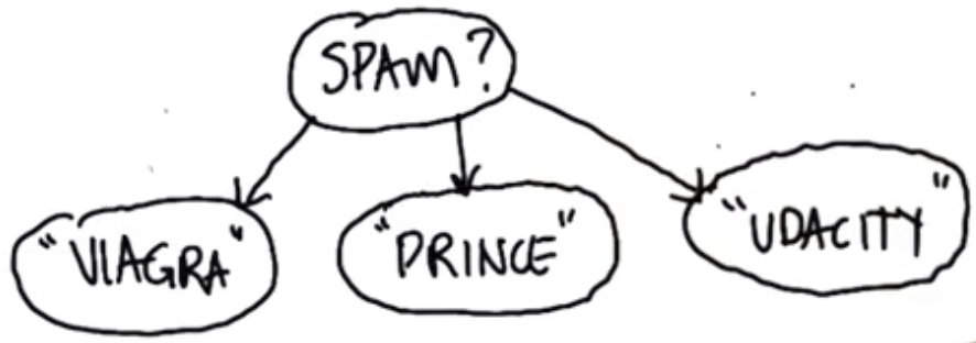
Naive Bayes is “naive” because it assumes that attributes are independent of one another, conditional on the label.
If a message is a spam email, it is likely to contain certain words.
| Which | True | False |
|---|---|---|
| $P(spam)$ | .4 | .6 |
| $P(“Viagra”|spam)$ | .3 | .001 |
| $P(“Price”|spam)$ | .2 | .1 |
| $P(“Udacity”|spam)$ | .0001 | .1 |
$$P(spam|“Viagra”,\ not\ “Prince”,\ not\ “Udacity”)=$$ $$=\frac{P(“Viagra”,\ not\ “Prince”,\ not\ “Udacity”)|spam}{…}$$ $$=\frac{P(“Viagra”|spam)P(not\ “Prince”)|spam)P(not\ “Udacity”|spam)P(spam)}{…}$$ $$=\frac{(.3)(.8)(.9999)(.4)}{…}$$
Naive Bayes - Generic Form
Using the previous example, the type of email can be considered as a class, $V$. The various words that are more common to spam emails can be considered specific examples of attributes, $a_1, a_2, … a_n$. $Z$ is the number of attributes, and is a normalizing term. Recall $\prod_i$ means take the product over $i$.
$$P(V|a_1, a_2, … a_n) = \prod_i \frac{P(\frac{a_i}{V}) P(V)}{Z}$$
If we have a way of generating attribute values from classes, then the foregoing formula allows us to go in the opposite direction. We can observe the attribute values and infer the class.
$$MAP\ class = argmax\lbrace P(V) \prod_i P(\frac{a_i}{V})\rbrace$$
Naive Bayes Benefits
- Inference is cheap
- Few parameters
- Estimate parameters with labeled data
- Connects inference and classification
- Empirically successful
- For example, widely employed at Google
For Fall 2019, CS 7461 is instructed by Dr. Charles Isbell. The course content was originally created by Dr. Charles Isbell and Dr. Michael Littman.