Model Overfitting
Overfitting is the situation where a model is trained on a certain set of data, but then does not work at all, or performs very poorly, with test data. This is especially a problem in today’s environment of very cheap computation, because its become so easy with computers to fit almost any data with a complex model. Fortunately, there are techniques that can be used to avoid overfitting.
One way to conceptualize overfitting is to consider what models most fundamentally are. Models are a way for analysts to extract signal from noise. With an overfit model, the analyst is overconfident about his model’s ability to extract signal from a mixture of signal and noise. The overfit model includes some of the noise in the training set data as if it were part of the signal, so the signal appears stronger than it actually is. As a result, the performance on the test data is worse than would otherwise be expected.
An Illustration
Professor Egger presents a series of correlations between randomly generated variables. For his experiment, 1000 samples of 25 random x and y values are generated. The correlations he found ranged from values less than -0.5 to greater than 0.5. Being perfectly random values, the actual correlation of the underlying variables, x and y, is zero.
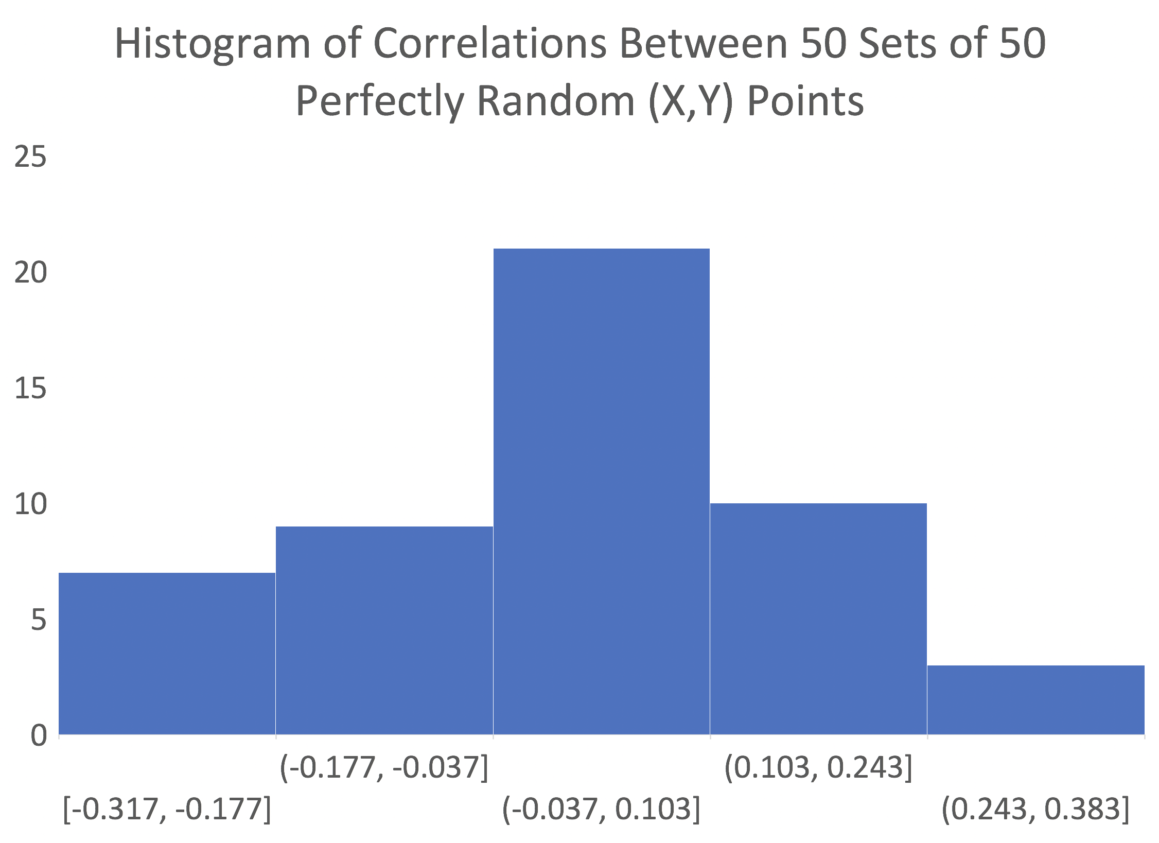
I produced 50 sets of 50 random (x,y) data points. A histogram of the correlations for these datasets is presented below. Being fewer datasets with a larger sample size, the effect is less pronounced, but correlations still range from -0.317 to 0.289.
Mathematical Explanation
Assume an ideal situation of simple linear regression with no overfitting. The process takes values $x_i$ and outputs values $y_i$. Assume $x_i$ and the errors are drawn from independent Gaussian distributions with $\sigma=1$, which means that the output, $y_i$, is also 1. These constraints are expressed mathematically below.
$$\beta=R=\sigma_{signal}$$
$$\sigma_x=\sigma_y=1$$
A perfect model (signal only, no noise) would be given by the following.
$$\hat{y_i}=\beta x_i$$
A model that includes error and describes this process is shown below.
$$y_i=\beta x_i+\phi(0,\sigma_e^2)$$
The signal is represented by $\beta x_i$ and the noise is represented by $\phi(0,\sigma_e^2)$.
The difference between $\hat{y_i}$ and $y_i$ is termed the residual. The standard deviation of the residual is the standard deviation of the error.
Source of Additional Overfitting Error
For simple statistical analyses, it is reasonable to assume, as shown above, that a best fit line has fixed parameters $\alpha$, $\beta$, and $\sigma_e$. In reality, however, each of those parameters (for a linear model generated from a small- to medium-sized set of ordered pairs) is only an estimate, which can be denoted $\hat{\alpha}$, $\hat{\beta}$, and $\hat{\sigma_e}$. In actuality, each of those parameters has their own error.
Given this, the true error for $y_i$ is not $\hat{\sigma_e}$, but some combination of all three errors outlined in the previous paragraph. There are mathematical methods for calculating each of those sources of error, but they are beyond the scope of this note.
The effect of overfitting is to exaggerate the effect of noise such that not only is our error greater than we expect, but it is actually greater than the true noise of the situation if we had a correct knowledge of the actual model. This explanation should give an intuitive reason for the process by which overfitting a model actually produces greater error than the true noise. In other words, overfitting makes the error even worse.
Numerical Example
Assume we have a process with true correlation, $R$, equals 0.50. Then, the standard deviation of random error would be
$$\sigma_e=\sqrt{(1-R^2)}=\sqrt{(1-.5^2)}=0.866$$
Further assume that this model was developed based upon a collection of ordered pairs, and the best fit line was given by $\hat{\beta}=0.85$. Again, the true $\beta=R=0.5$, but we would believe that the correlation, $R$, equaled 0.85. Then, the believed error would be given by the
$$\sigma_{e,believed}=\sqrt{1-.85^2}=0.527$$
So, the true error is much larger than we expected based on the overfit model.
$$\frac{\sigma_e}{\sigma_{e,believed}}=\frac{0.866}{0.527}=1.64$$
In fact, 64% larger.
It gets worse. The error is actually dependent upon the specific value of $x_i$. So, for example, consider the point at $x_i = 2$. At that point,
$$y_i=\beta x_i=(.5)(2)=1$$
But,
$$\hat{y_i}=\hat{\beta} x_i=(.85)(2)=1.7$$
So the error at that point is $1.7-1=0.7$. The error is $x_i$ multiplied by the delta between the true slope and the believed slope. So, this additional error is given by
$$\phi(0,(\hat{\beta}-\beta)^2)$$
Or, in this case
$$\phi(0,.35^2)$$
Adding this new error to the previous estimate gives us
$$\sqrt{.866^2+.35^2}=0.93$$
So the new total error is
$$\frac{\sigma_e}{\sigma_{e,believed}}=\frac{0.93}{0.527}=1.77$$
Or, 77% higher than expected. This is the penalty paid for overfitting.
Conclusion
After training a model on a training set with a modest amount of data, if a high correlation is obtained, it is very likely that the true correlation is lower than the initial estimate. A much lower correlation on a test set of data is a sure sign of overfitting. The closer a correlation estimate on a test data set is to the training correlation estimate, the more likely it is that both estimates are relative close to the true value of the signal.
As general guidelines, standard deviations of model error that exhibit:
- an increase of less than 20% suggests minimal model over-fitting.
- an increase of more than 25% suggests possible model over-fitting.
- an increase of more than 50% leads to the conclusion of model over-fitting.