Engineering a Metric for a Binary Classifier
Consider the following practical example of binary classification. For a single day, a hypothetical bank issues credit cards to everyone who applies, and monitors the performance of the resulting loans. The dataset the class is provided includes two sets of 200 fictitious customers, one of which is “training” data and the other of which is “testing” data. The first few rows of this data are presented below.
As part of the normal process of issuing loans, for each customer, the hypothetical bank captures the information shown below. A 1 in the Outcome column indicates that the customer defaulted.
| Age | Years at Employer | Years at Address | Income | Credit Card Debt | Automobile Debt | Outcome |
|---|---|---|---|---|---|---|
| 32.53 | 9.39 | 0.30 | $37,844 | -$3,247 | -$4,795 | 0 |
| 34.58 | 11.97 | 1.49 | $65,765 | -$15,598 | -$17,632 | 1 |
| 37.70 | 12.46 | 0.09 | $61,002 | -$11,402 | -$7,910 | 1 |
Engineering a Composite Metric
The AUC for each of these individual parameters, using the training data, is tabulated below.
| Age | Years at Employer | Years at Address | Income | Credit Card Debt | Automobile Debt |
|---|---|---|---|---|---|
| 0.64 | 0.72 | 0.58 | 0.63 | 0.60 | 0.62 |
It is reasonable to assume that the ratio of total debt to income would be predictive of a customer’s ability to repay loans. This is calculated as follows.
$$\frac{Debt}{Income} = \frac{|Credit\ Card\ Debt + Auto\ Debt|}{Income}$$
This debt-to-income metric is a much stronger predictor of whether a customer will default than any of the individual metrics. Using the training data, it results in an AUC of 0.74.
Note, still, that Years at Employer is still nearly as strong a predictor on its own. It seems appropriate to combine these two metrics to see if, combined, they might produce something stronger overall. The values must be standardized before being combined. Years at Employer is negatively correlated with likelihood of default, whereas debt-to-income is positively correlated. Thus, they are combined as follows, where std indicates the data are standardized.
$$Metric = std(\frac{Debt}{Income})-std(Years\ at\ Employer)$$
Or:
$$Metric = std(\frac{|Credit\ Card\ Debt + Auto\ Debt|}{Income})-std(Years\ at\ Employer)$$
Using the training data, this composite metric results in an AUC of 0.82.
The data are developed piecemeal, below. First, the raw data are used to calculate the $\frac{debt}{inc}$ ratio.
| Income | CC Debt | Auto Debt | Debt/Inc Ratio | Years at Employer |
|---|---|---|---|---|
| $37,844 | -$3,247 | -$4,795 | 21% | 9.39 |
| $65,765 | -$15,598 | -$17,632 | 51% | 11.97 |
| $61,002 | -$11,402 | -$7,910 | 32% | 12.46 |
Then, the $\frac{debt}{inc}$ and $Years\ at\ Employer$ are standardized and the results subtracted. Finally, that composite metric is itself standardized.
| Std Debt/Inc | Std Years at Employer | Composite Metric | Std Composite Metric |
|---|---|---|---|
| 0.04 | 0.11 | -0.08 | -0.05 |
| 2.00 | 0.50 | 1.51 | 1.03 |
| 0.74 | 0.57 | 0.17 | 0.11 |
Performance of the Metric
When tested using a set of testing data, this classification scheme produces the results below.
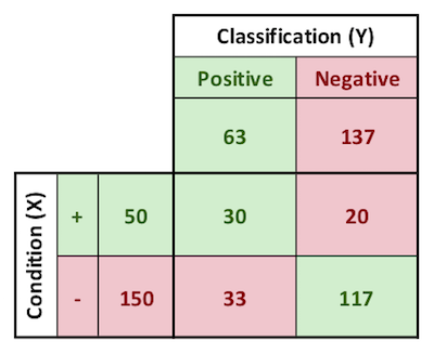
A: p(+), incidence of + condition
B: p(-), incidence of - condition
C: p(test POS), incidence of POS classification
D: p(test NEG), incidence of NEG classification
E: p(test POS, +), true positives
F: p(test NEG, +), false negatives
G: p(test POS, -), false positives
H: p(test NEG, -), true negatives
With parameters expressed as probabilities, the matrix is as shown below.
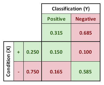
$$\text{true positive count} = p(test\ POS,\ +) = E = .150$$
$$\text{true positive rate} = p(test\ POS\ | +) \ = \frac{E}{A} = \frac{.150}{.250} = .600$$
$$\text{positive predictive value} = p(+ | test\ POS) \ = \frac{E}{C} = \frac{.150}{.315} = .480$$
Binary-Performance-Metrics.xlsx
Review-of-AUC-for-ROC-Curve.xlsx
Forecasting-Soldier-Performance.xlsx
AUC_Calculator-and-Review-of-AUC-Curve.xlsx
Data_Final-Project.xlsx
Information-Gain-Calculator.xlsx
Some other content is taken from my notes on other aspects of the aforementioned Coursera course.