Unsupervised Learning to Identify Customer Segments
In this project, I apply unsupervised machine learning techniques to better understand the core core customer base for a mail-order sales company in Germany.
The project involved segmenting large, high-dimensional data related the German population. By comparing similar data for customers of the company, I determined which population segments are disproportionately represented among the company’s customers. These insights could be used to direct marketing campaigns towards audiences that are most likely to be responsive.
The result of the project was a clearer understanding of the company’s typical customer. Specifically, the analysis showed that the company’s customer base is disproportionately financially thrify, relatively old, dutiful, religious, and traditional.
The data used was provided by Udacity partner Bertelsmann Arvato Analytics.
This is page 2 of 2 for the project, where I
Transform Features and Cluster the Data
The specific tasks break down as follows:
- 1: Feature Transformation
- 1.1: Apply Feature Scaling
- 1.2: Perform Dimensionality Reduction
- 1.3: Interpret Principal Components
- 2: Clustering
- 2.1: Apply Clustering to General Population
- 3: Apply All Steps to the Customer Data
- 3.1: Feature Scaling
- 3.2: Dimensionality Reduction
- 3.3: Clustering
- 4: Compare Customer Data to Demographics Data
- 5: Discuss Results
1. Feature Transformation
The raw demographics and customers data was cleansed and preprocessed on the previous page of this project. It was saved as a_processed.csv and c_processed.csv.
import numpy as np
import pandas as pd
import matplotlib.pyplot as plt
import seaborn as sns
from sklearn.preprocessing import StandardScaler
from sklearn.decomposition import PCA
from sklearn.cluster import KMeans
Preprocessed Demographics Data
a_path = '/home/ryan/large-files/datasets/customer-segments/processed/a_processed.csv'
a = pd.read_csv(a_path, index_col=0)
print(a.shape)
print(str(a.isna().sum().sum()) + ' missing values')
a.head()
(623211, 179)
0 missing values
| ALTERSKATEGORIE_GROB | FINANZ_MINIMALIST | FINANZ_SPARER | FINANZ_VORSORGER | FINANZ_ANLEGER | FINANZ_UNAUFFAELLIGER | FINANZ_HAUSBAUER | HEALTH_TYP | RETOURTYP_BK_S | SEMIO_SOZ | ... | ZABEOTYP_4.0 | ZABEOTYP_5.0 | ZABEOTYP_6.0 | NATIONALITAET_KZ_1.0 | NATIONALITAET_KZ_2.0 | NATIONALITAET_KZ_3.0 | PRAEGENDE_JUGENDJAHRE_decade | PRAEGENDE_JUGENDJAHRE_movement | CAMEO_INTL_2015_wealth | CAMEO_INTL_2015_life_stage | |
|---|---|---|---|---|---|---|---|---|---|---|---|---|---|---|---|---|---|---|---|---|---|
| 0 | 1.0 | 1.0 | 5.0 | 2.0 | 5.0 | 4.0 | 5.0 | 3.0 | 1.0 | 5.0 | ... | 0 | 1 | 0 | 1 | 0 | 0 | 6.0 | 0.0 | 5.0 | 1.0 |
| 1 | 3.0 | 1.0 | 4.0 | 1.0 | 2.0 | 3.0 | 5.0 | 3.0 | 3.0 | 4.0 | ... | 0 | 1 | 0 | 1 | 0 | 0 | 6.0 | 1.0 | 2.0 | 4.0 |
| 2 | 3.0 | 4.0 | 3.0 | 4.0 | 1.0 | 3.0 | 2.0 | 3.0 | 5.0 | 6.0 | ... | 1 | 0 | 0 | 1 | 0 | 0 | 4.0 | 0.0 | 4.0 | 3.0 |
| 3 | 1.0 | 3.0 | 1.0 | 5.0 | 2.0 | 2.0 | 5.0 | 3.0 | 3.0 | 2.0 | ... | 1 | 0 | 0 | 1 | 0 | 0 | 2.0 | 0.0 | 5.0 | 4.0 |
| 4 | 2.0 | 1.0 | 5.0 | 1.0 | 5.0 | 4.0 | 3.0 | 2.0 | 4.0 | 2.0 | ... | 1 | 0 | 0 | 1 | 0 | 0 | 5.0 | 0.0 | 2.0 | 2.0 |
5 rows × 179 columns
1.1. Apply Feature Scaling
Default StandardScaler fits each feature to mean 0 and standard deviation 1.
scalar = StandardScaler()
a_ss = scalar.fit_transform(a)
a = pd.DataFrame(a_ss,
                 columns=a.columns)
a.head()
| ALTERSKATEGORIE_GROB | FINANZ_MINIMALIST | FINANZ_SPARER | FINANZ_VORSORGER | FINANZ_ANLEGER | FINANZ_UNAUFFAELLIGER | FINANZ_HAUSBAUER | HEALTH_TYP | RETOURTYP_BK_S | SEMIO_SOZ | ... | ZABEOTYP_4.0 | ZABEOTYP_5.0 | ZABEOTYP_6.0 | NATIONALITAET_KZ_1.0 | NATIONALITAET_KZ_2.0 | NATIONALITAET_KZ_3.0 | PRAEGENDE_JUGENDJAHRE_decade | PRAEGENDE_JUGENDJAHRE_movement | CAMEO_INTL_2015_wealth | CAMEO_INTL_2015_life_stage | |
|---|---|---|---|---|---|---|---|---|---|---|---|---|---|---|---|---|---|---|---|---|---|
| 0 | -1.746287 | -1.512226 | 1.581061 | -1.045045 | 1.539061 | 1.047076 | 1.340485 | 1.044646 | -1.665693 | 0.388390 | ... | -0.609065 | 2.966193 | -0.309313 | 0.383221 | -0.307557 | -0.208434 | 1.164455 | -0.553672 | 1.147884 | -1.251111 |
| 1 | 0.202108 | -1.512226 | 0.900446 | -1.765054 | -0.531624 | 0.318375 | 1.340485 | 1.044646 | -0.290658 | -0.123869 | ... | -0.609065 | 2.966193 | -0.309313 | 0.383221 | -0.307557 | -0.208434 | 1.164455 | 1.806125 | -0.909992 | 0.749820 |
| 2 | 0.202108 | 0.692400 | 0.219832 | 0.394972 | -1.221852 | 0.318375 | -0.856544 | 1.044646 | 1.084378 | 0.900649 | ... | 1.641861 | -0.337133 | -0.309313 | 0.383221 | -0.307557 | -0.208434 | -0.213395 | -0.553672 | 0.461926 | 0.082843 |
| 3 | -1.746287 | -0.042475 | -1.141397 | 1.114980 | -0.531624 | -0.410325 | 1.340485 | 1.044646 | -0.290658 | -1.148386 | ... | 1.641861 | -0.337133 | -0.309313 | 0.383221 | -0.307557 | -0.208434 | -1.591245 | -0.553672 | 1.147884 | 0.749820 |
| 4 | -0.772089 | -1.512226 | 1.581061 | -1.765054 | 1.539061 | 1.047076 | -0.124201 | -0.273495 | 0.396860 | -1.148386 | ... | 1.641861 | -0.337133 | -0.309313 | 0.383221 | -0.307557 | -0.208434 | 0.475530 | -0.553672 | -0.909992 | -0.584134 |
5 rows × 179 columns
1.2. Perform Dimensionality Reduction
The following helper function fits sklearn’s Principal Component Analysis PCA library on the scaled data using the specified number of components. It returns the actual PCA object as well as the fit data.
def do_pca(n_components, data):
    pca = PCA(n_components)
    X_pca = pca.fit_transform(data)
    X_pca = pd.DataFrame(X_pca)
    return pca, X_pca
The following helper plots the amount of variance explained by each component.
def scree_plot(pca):
    num_components = len(pca.explained_variance_ratio_)
    ind = np.arange(num_components)
    vals = pca.explained_variance_ratio_

    plt.figure(figsize=(14, 7))
    ax = plt.subplot(111)
    cumvals = np.cumsum(vals)
    ax.bar(ind, vals)
    ax.plot(ind, cumvals, color='darkorange')

    if num_components <= 30:
        for i in range(num_components):
            ax.annotate(r"%s%%" % ((str(round(vals[i]*100,1))[:3])),
                        (ind[i]+0.2, vals[i]),
                        va="bottom",
                        ha="center",
                        fontsize=8)

    ax.xaxis.set_tick_params(width=0)
    ax.yaxis.set_tick_params(width=1, length=6)

    ax.set_xlabel("Principal Component")
    ax.set_ylabel("Variance Explained (%)")

    for spine in ax.spines.values():
        spine.set_visible(False)

    plt.title('Explained Variance Per Principal Component')
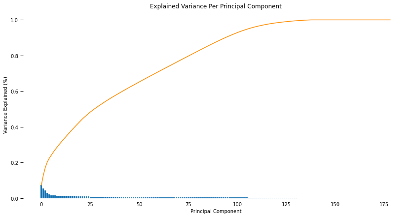
pca_182, a_pca = do_pca(a.shape[1], a)
scree_plot(pca_182)

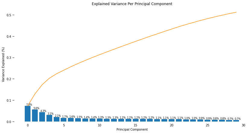
The first 30 principal components appear to explain roughly 50% of the overall variance.
pca, a_pca = do_pca(30, a)
scree_plot(pca)

1.3. Interpret Principal Components
Now that we have our transformed principal components, it’s a nice idea to check out the weight of each variable on the first few components to see if they can be interpreted in some fashion.
As a reminder, each principal component is a unit vector that points in the direction of highest variance (after accounting for the variance captured by earlier principal components). The further a weight is from zero, the more the principal component is in the direction of the corresponding feature. If two features have large weights of the same sign (both positive or both negative), then increases in one tend expect to be associated with increases in the other. To contrast, features with different signs can be expected to show a negative correlation: increases in one variable should result in a decrease in the other.
The following helper function creates a results DataFrame with the feature weights.
def pca_results(full_dataset, pca):
    # Dimension indexing
    dimensions = dimensions = \
    ['Dimension {}'.format(i) for i in range(1,len(pca.components_)+1)]

    # PCA components
    components = pd.DataFrame(np.round(pca.components_, 4),
                              columns = full_dataset.keys())
    components.index = dimensions

    # PCA explained variance
    ratios = pca.explained_variance_ratio_.reshape(len(pca.components_), 1)
    variance_ratios = pd.DataFrame(np.round(ratios, 4),
                                   columns = ['Explained Variance'])
    variance_ratios.index = dimensions

    # Return a concatenated DataFrame
    return (pd.concat([variance_ratios, components],
                      axis = 1))
results = pca_results(a, pca)
print(results.shape)
results.T[['Dimension 1','Dimension 2','Dimension 3']].head()
(30, 180)
| Dimension 1 | Dimension 2 | Dimension 3 | |
|---|---|---|---|
| Explained Variance | 0.0732 | 0.0557 | 0.0430 |
| ALTERSKATEGORIE_GROB | 0.2145 | -0.1243 | 0.0587 |
| FINANZ_MINIMALIST | 0.2184 | 0.0940 | 0.0845 |
| FINANZ_SPARER | -0.2297 | 0.0920 | -0.0701 |
| FINANZ_VORSORGER | 0.2002 | -0.1027 | 0.0720 |
The following helper function sorts the results DataFrame to show the most important features for each dimension.
def top_features(dimension, count=5):
    col_label = 'Dimension {}'.format(dimension)

    most_positive = (results
                     .drop(columns=['Explained Variance'])
                     .T
                     [[col_label]]
                     .sort_values([col_label], ascending=False)
                     .head(count))

    most_negative = (results
                     .drop(columns=['Explained Variance'])
                     .T
                     [[col_label]]
                     .sort_values([col_label], ascending=False)
                     .tail(count))

    top_features = most_positive.append(most_negative)

    return top_features
Dimension 1
top_1 = top_features(1)
top_1
| Dimension 1 | |
|---|---|
| FINANZ_MINIMALIST | 0.2184 |
| ALTERSKATEGORIE_GROB | 0.2145 |
| FINANZ_VORSORGER | 0.2002 |
| SEMIO_LUST | 0.1543 |
| SEMIO_ERL | 0.1502 |
| SEMIO_TRADV | -0.1830 |
| SEMIO_REL | -0.1906 |
| SEMIO_PFLICHT | -0.1958 |
| PRAEGENDE_JUGENDJAHRE_decade | -0.2030 |
| FINANZ_SPARER | -0.2297 |
Interpretation of Dimension 1
- People who are financially thrify, financially disinterested, relatively older, dutiful, religious, and traditional.
Detailed feature breakdown:
Direction of Vector:
- FINANZ_MINIMALIST: Financial typology, for each dimension: low financial interest
- 1: very high
- …
- 5: very low
- ALTERSKATEGORIE_GROB: Estimated age based on given name analysis
- 1: < 30 years old
- …
- 4: > 60 years old
- FINANZ_VORSORGER: Financial typology, for each dimension: be prepared
- SEMIO_LUST: Personality typology, for each dimension: sensual-minded
- 1: highest affinity
- …
- 7: lowest affinity
- SEMIO_ERL: Personality typology, for each dimension: event-oriented
Opposite Direction:
- SEMIO_TRADV: Personality typology, for each dimension: tradional-minded
- SEMIO_REL: Personality typology, for each dimension: religious
- SEMIO_PFLICHT: Personality typology, for each dimension: dutiful
- PRAEGENDE_JUGENDJAHRE_decade: Dominating movement of person’s youth (avantgarde vs. mainstream; east vs. west): decade of event
- 1: 40s - war years (Mainstream, E+W)
- 2: 40s - reconstruction years (Avantgarde, E+W)
- …
- 14: 90s - digital media kids (Mainstream, E+W)
- 15: 90s - ecological awareness (Avantgarde, E+W)
- FINANZ_SPARER: Financial typology, for each dimension: money-saver
Dimension 2
top_2 = top_features(2)
top_2
| Dimension 2 | |
|---|---|
| ONLINE_AFFINITAET | 0.1715 |
| SEMIO_KULT | 0.1641 |
| SEMIO_REL | 0.1570 |
| ZABEOTYP_1.0 | 0.1565 |
| ANZ_PERSONEN | 0.1356 |
| SEMIO_ERL | -0.1630 |
| ZABEOTYP_3.0 | -0.1658 |
| CAMEO_INTL_2015_wealth | -0.1746 |
| HH_EINKOMMEN_SCORE | -0.1778 |
| FINANZ_HAUSBAUER | -0.1861 |
Interpretation of Dimension 2
- People who are home-owners, high income, wealthy, have a high affinity for being online, and are “green” in terms of energy consumption.
Detailed feature breakdown:
Direction of Vector:
- ONLINE_AFFINITAET: Online affinity
- 0: none
- 5: highest
- SEMIO_KULT: Personality typology, for each dimension: cultural-minded
- 1: highest affinity
- …
- 7: lowest affinity
- SEMIO_REL: Personality typology, for each dimension: religious
- ZABEOTYP_1.0: Energy consumption typology: green
- ANZ_PERSONEN: Number of adults in household
Opposite Direction:
- SEMIO_ERL: Personality typology, for each dimension: event-oriented
- ZABEOTYP_3.0: Energy consumption typology: fair supplied
- CAMEO_INTL_2015_wealth: German CAMEO: Wealth / Life Stage Typology, mapped to international code: Wealth
- 1: Wealthy
- …
- 5: Poorer
- HH_EINKOMMEN_SCORE: Estimated household net income
- 1: highest income
- 6: very low income
- FINANZ_HAUSBAUER: Financial typology, for each dimension: home owndership
Dimension 3
top_3 = top_features(3)
top_3
| Dimension 3 | |
|---|---|
| ANREDE_KZ_1.0 | 0.3151 |
| SEMIO_VERT | 0.2851 |
| SEMIO_SOZ | 0.2259 |
| SEMIO_FAM | 0.2255 |
| SEMIO_KULT | 0.2043 |
| SEMIO_RAT | -0.1764 |
| SEMIO_KRIT | -0.2134 |
| SEMIO_DOM | -0.2560 |
| SEMIO_KAEM | -0.2759 |
| ANREDE_KZ_2.0 | -0.3151 |
Interpretation of Dimension 3
- Males who are personally combative, dominant, critical, and rational. They are specifically not dreamful, socially-minded, family-minded, or culturally-minded.
Detailed feature breakdown:
Direction of Vector:
- ANREDE_KZ_1.0: Male Gender
- SEMIO_VERT: Personality typology, for each dimension: dreamful
- 1: highest affinity
- …
- 7: lowest affinity
- SEMIO_SOZ: Personality typology, for each dimension: socially-minded
- SEMIO_FAM: Personality typology, for each dimension: family-minded
- SEMIO_KULT: Personality typology, for each dimension: cultural-minded
Opposite Direction:
- SEMIO_RAT: Personality typology, for each dimension: rational
- SEMIO_KRIT: Personality typology, for each dimension: critical-minded
- SEMIO_DOM: Personality typology, for each dimension: dominant-minded
- SEMIO_KAEM: Personality typology, for each dimension: combative attitude
- ANREDE_KZ_2.0: Female Gender
2. Clustering
2.1. Apply Clustering to General Population
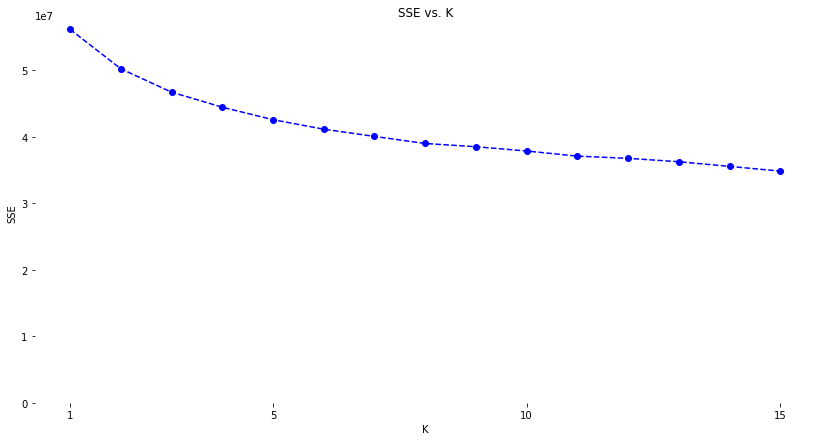
Now, check and see how the data clusters in the principal components step. In this step, I apply k-means clustering to the dataset and use the “elbow method” to determine the optimal number of clusters to use.
scores = []
centers = list(range(1,16))
for center in centers:
    kmeans = KMeans(n_clusters=center)
    model = kmeans.fit(a_pca)
    score = np.abs(model.score(a_pca))
    scores.append(score)
plt.figure(figsize=(14, 7))
plt.plot(centers, scores, linestyle='--', marker='o', color='b')
plt.ylim(bottom=0)
plt.xlabel('K')
plt.xticks([1,5,10,15])
plt.ylabel('SSE')
plt.title('SSE vs. K')
for spine in plt.gca().spines.values():
    spine.set_visible(False)

Based on the plot above, I select 5 as a resonable point of diminishing returns.
kmeans = KMeans(n_clusters=5)
model = kmeans.fit(a_pca)
a_labels = (pd.DataFrame(model.predict(a_pca))
            .rename(columns={0:'demo label'}))
print(a_labels.shape)
(623211, 1)
a_label_counts = (pd.DataFrame(a_labels['demo label'].value_counts())
                  .rename(columns={'demo label':'demo count'}))
a_label_counts['demo percent'] = round(a_label_counts['demo count'] /
                                       a_labels.shape[0]*100,1)
3. Apply All Steps to the Customer Data
Next, I apply all these steps to the cleansed customer data using the same, fitted skelarn models generated above.
c_path = '/home/ryan/large-files/datasets/customer-segments/processed/c_processed.csv'
c = pd.read_csv(c_path, index_col=0)
print(c.shape)
print(str(c.isna().sum().sum()) + ' missing values')
c.head()
(133377, 179)
0 missing values
| ALTERSKATEGORIE_GROB | FINANZ_MINIMALIST | FINANZ_SPARER | FINANZ_VORSORGER | FINANZ_ANLEGER | FINANZ_UNAUFFAELLIGER | FINANZ_HAUSBAUER | HEALTH_TYP | RETOURTYP_BK_S | SEMIO_SOZ | ... | ZABEOTYP_4.0 | ZABEOTYP_5.0 | ZABEOTYP_6.0 | NATIONALITAET_KZ_1.0 | NATIONALITAET_KZ_2.0 | NATIONALITAET_KZ_3.0 | PRAEGENDE_JUGENDJAHRE_decade | PRAEGENDE_JUGENDJAHRE_movement | CAMEO_INTL_2015_wealth | CAMEO_INTL_2015_life_stage | |
|---|---|---|---|---|---|---|---|---|---|---|---|---|---|---|---|---|---|---|---|---|---|
| 0 | 4.0 | 5.0 | 1.0 | 5.0 | 1.0 | 2.0 | 2.0 | 1.0 | 5.0 | 6.0 | ... | 0 | 0 | 0 | 1 | 0 | 0 | 2.0 | 1.0 | 1.0 | 3.0 |
| 1 | 4.0 | 5.0 | 1.0 | 5.0 | 1.0 | 4.0 | 4.0 | 2.0 | 5.0 | 2.0 | ... | 0 | 0 | 0 | 1 | 0 | 0 | 2.0 | 1.0 | 3.0 | 4.0 |
| 2 | 4.0 | 5.0 | 1.0 | 5.0 | 2.0 | 1.0 | 2.0 | 2.0 | 3.0 | 6.0 | ... | 0 | 0 | 0 | 1 | 0 | 0 | 1.0 | 0.0 | 2.0 | 4.0 |
| 3 | 3.0 | 3.0 | 1.0 | 4.0 | 4.0 | 5.0 | 2.0 | 3.0 | 5.0 | 4.0 | ... | 0 | 0 | 0 | 1 | 0 | 0 | 4.0 | 0.0 | 4.0 | 1.0 |
| 4 | 3.0 | 5.0 | 1.0 | 5.0 | 1.0 | 2.0 | 3.0 | 3.0 | 3.0 | 6.0 | ... | 0 | 0 | 0 | 1 | 0 | 0 | 2.0 | 1.0 | 3.0 | 4.0 |
5 rows × 179 columns
3.1. Feature Scaling
c_ss = scalar.transform(c)
c = pd.DataFrame(c_ss,
                 columns=c.columns)
print(c.shape)
c.head()
(133377, 179)
| ALTERSKATEGORIE_GROB | FINANZ_MINIMALIST | FINANZ_SPARER | FINANZ_VORSORGER | FINANZ_ANLEGER | FINANZ_UNAUFFAELLIGER | FINANZ_HAUSBAUER | HEALTH_TYP | RETOURTYP_BK_S | SEMIO_SOZ | ... | ZABEOTYP_4.0 | ZABEOTYP_5.0 | ZABEOTYP_6.0 | NATIONALITAET_KZ_1.0 | NATIONALITAET_KZ_2.0 | NATIONALITAET_KZ_3.0 | PRAEGENDE_JUGENDJAHRE_decade | PRAEGENDE_JUGENDJAHRE_movement | CAMEO_INTL_2015_wealth | CAMEO_INTL_2015_life_stage | |
|---|---|---|---|---|---|---|---|---|---|---|---|---|---|---|---|---|---|---|---|---|---|
| 0 | 1.176305 | 1.427276 | -1.141397 | 1.114980 | -1.221852 | -0.410325 | -0.856544 | -1.591635 | 1.084378 | 0.900649 | ... | -0.609065 | -0.337133 | -0.309313 | 0.383221 | -0.307557 | -0.208434 | -1.591245 | 1.806125 | -1.595951 | 0.082843 |
| 1 | 1.176305 | 1.427276 | -1.141397 | 1.114980 | -1.221852 | 1.047076 | 0.608142 | -0.273495 | 1.084378 | -1.148386 | ... | -0.609065 | -0.337133 | -0.309313 | 0.383221 | -0.307557 | -0.208434 | -1.591245 | 1.806125 | -0.224033 | 0.749820 |
| 2 | 1.176305 | 1.427276 | -1.141397 | 1.114980 | -0.531624 | -1.139026 | -0.856544 | -0.273495 | -0.290658 | 0.900649 | ... | -0.609065 | -0.337133 | -0.309313 | 0.383221 | -0.307557 | -0.208434 | -2.280170 | -0.553672 | -0.909992 | 0.749820 |
| 3 | 0.202108 | -0.042475 | -1.141397 | 0.394972 | 0.848833 | 1.775776 | -0.856544 | 1.044646 | 1.084378 | -0.123869 | ... | -0.609065 | -0.337133 | -0.309313 | 0.383221 | -0.307557 | -0.208434 | -0.213395 | -0.553672 | 0.461926 | -1.251111 |
| 4 | 0.202108 | 1.427276 | -1.141397 | 1.114980 | -1.221852 | -0.410325 | -0.124201 | 1.044646 | -0.290658 | 0.900649 | ... | -0.609065 | -0.337133 | -0.309313 | 0.383221 | -0.307557 | -0.208434 | -1.591245 | 1.806125 | -0.224033 | 0.749820 |
5 rows × 179 columns
3.2. Dimensionality Reduction
c_pca = pca.transform(c)
c_pca = pd.DataFrame(c_pca)
print(c_pca.shape)
c_pca.head()
(133377, 30)
| 0 | 1 | 2 | 3 | 4 | 5 | 6 | 7 | 8 | 9 | ... | 20 | 21 | 22 | 23 | 24 | 25 | 26 | 27 | 28 | 29 | |
|---|---|---|---|---|---|---|---|---|---|---|---|---|---|---|---|---|---|---|---|---|---|
| 0 | 7.058972 | 3.420497 | 2.500324 | 2.100575 | -0.997242 | 0.357982 | 1.643074 | -1.987261 | -0.131893 | 3.745730 | ... | -2.629017 | -3.100104 | -1.653428 | 1.266194 | -1.564352 | -1.139092 | 0.593162 | -0.507610 | -0.417441 | -0.898603 |
| 1 | 5.527108 | -2.299668 | -1.057538 | 4.004213 | -3.509783 | 0.377007 | -0.706439 | 0.596483 | 0.403730 | -0.726155 | ... | 2.007500 | -1.508163 | 1.866077 | 1.669437 | -0.639520 | 0.501114 | -1.797476 | 1.960346 | -1.062995 | 1.349571 |
| 2 | 3.965549 | 2.526799 | 1.897971 | -4.488827 | -0.490012 | -0.328013 | -1.467358 | -0.244206 | -0.963943 | 1.767246 | ... | -0.256628 | 1.314349 | 1.159087 | -0.805965 | -0.282223 | -1.838544 | 0.288024 | 1.200617 | 0.077224 | 0.680797 |
| 3 | -0.952263 | 1.129877 | 1.647568 | 0.479191 | 2.608330 | 0.865320 | -3.497100 | -0.222191 | -1.224088 | -0.148981 | ... | -0.071952 | -0.157687 | 0.032621 | -0.235610 | -2.169996 | -0.179192 | -3.537217 | 0.913882 | -0.013844 | -1.198688 |
| 4 | 3.920457 | 2.322970 | 2.579195 | 3.451799 | 0.253436 | 3.131984 | -1.969115 | 2.462193 | 3.717401 | 2.315231 | ... | 1.433696 | -1.553335 | 1.425058 | -1.520453 | 1.390906 | 5.829346 | 0.425688 | 1.927881 | -0.090094 | -0.447725 |
5 rows × 30 columns
3.3. Clustering
c_labels = model.predict(c_pca)
c_labels = (pd.DataFrame(c_labels)
            .rename(columns={0:'cust label'}))
print(c_labels.shape)
c_labels.head()
(133377, 1)
| cust label | |
|---|---|
| 0 | 2 |
| 1 | 2 |
| 2 | 0 |
| 3 | 4 |
| 4 | 2 |
c_label_counts = (pd.DataFrame(c_labels['cust label'].value_counts())
                  .rename(columns={'cust label':'cust count'}))
c_label_counts['cust percent'] = round(c_label_counts['cust count']/c_labels.shape[0]*100,
                                       1)
c_label_counts
| cust count | cust percent | |
|---|---|---|
| 2 | 62982 | 47.2 |
| 0 | 37226 | 27.9 |
| 1 | 27909 | 20.9 |
| 4 | 3026 | 2.3 |
| 3 | 2234 | 1.7 |
4. Compare Customer Data to Demographics Data
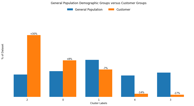
In this step, I compare the two cluster distributions to see where the strongest customer base for the company is.
cluster_counts = a_label_counts.join(c_label_counts)
cluster_counts['delta percent'] = (cluster_counts['cust percent'] -
                                   cluster_counts['demo percent'])
cluster_counts = (cluster_counts
                  .sort_values(['delta percent'],
                               ascending=False)
                  .reset_index()
                  .rename(columns={'index':'clusters'}))
cluster_counts['delta str'] = (cluster_counts['delta percent']
                               .round(0)
                               .astype(int)
                               .astype(str))
cluster_counts.loc[cluster_counts['delta percent']>0,
                 'delta str'] = '+' + cluster_counts['delta str']
cluster_counts['delta str'] = cluster_counts['delta str'] + '%'
ordered_cluster_list = list(cluster_counts['clusters'])
ordered_cluster_list
[2, 0, 1, 4, 3]
plt.figure(figsize=(14,7))
plt.bar(cluster_counts.index-0.1875,
        cluster_counts['demo percent'],
        width=0.375,
        label='General Population')
plt.bar(cluster_counts.index+0.1875,
        cluster_counts['cust percent'],
        width=0.375,
        label='Customer')
plt.xticks(range(0,len(cluster_counts)),
           cluster_counts['clusters'])
plt.ylim([0,70])
for spine in plt.gca().spines.values():
    spine.set_visible(False)
plt.xlabel('Cluster Labels')
plt.ylabel('% of Dataset')
plt.legend(fancybox=True,
           loc=9,
           ncol=4,
           facecolor='white',
           edgecolor='white',
           framealpha=1,
           fontsize=12)
plt.tick_params(
    axis='y',
    left=False,
    right=False,
    labelleft=False)
plt.tick_params(
    axis='x',
    bottom=False)
rects = plt.gca().patches[len(cluster_counts):]
deltas = list(cluster_counts['delta str'].values)
for n, r in enumerate(rects):
    height = r.get_height()
    plt.gca().text(r.get_x() + r.get_width() / 2,
                   height+1.2,
                   str(deltas[n]),
                   ha='center',
                   va='center')
plt.title('General Population Demographic Groups versus Customer Groups');

cust_median_centroids = (c_pca.join(c_labels)
                         .groupby('cust label')
                         .median()
                         .T)
cust_median_centroids.columns.name = 'pc'
cust_median_centroids = (cust_median_centroids[ordered_cluster_list]
                         .round(1))
print(cust_median_centroids.shape)
cust_median_centroids.index += 1
cust_median_centroids.head()
(30, 5)
| pc | 2 | 0 | 1 | 4 | 3 |
|---|---|---|---|---|---|
| 1 | 4.9 | 3.8 | 2.0 | -1.8 | -2.5 |
| 2 | 2.8 | 1.6 | -3.1 | 2.2 | -0.4 |
| 3 | 1.8 | 0.9 | 1.0 | 2.5 | -3.0 |
| 4 | 3.0 | -2.9 | 0.5 | 0.3 | 0.8 |
| 5 | 0.3 | 1.2 | 0.1 | 0.5 | 0.2 |
The following helper function determines the top number of most important components in each cluster.
def most_important_components(df, cluster, top=2):
    high = (cust_median_centroids
            .sort_values([cluster],
                         ascending=False)
            [:top]
            [[cluster]])
    low = (cust_median_centroids
           .sort_values([cluster],
                        ascending=False)
           [-1*top:]
           [[cluster]])
    combined = (high
                .append(low))
    combined['abs'] = combined[cluster].abs()
    combined = (combined
                .sort_values(['abs'],
                             ascending=False)
                .drop(columns=['abs']))
    return combined
The following table shows the most important principal component vectors that characterize each of the 5 clusters. The most important principal components can be either in the direction of a component or strongly opposite (negative).
top = 3
top_components_across_clusters = most_important_components(cust_median_centroids,
                                                           ordered_cluster_list[0],
                                                           top)

for cluster in ordered_cluster_list[1:]:
    next_cluster = most_important_components(cust_median_centroids,
                                             cluster,
                                             top)
    top_components_across_clusters = (top_components_across_clusters
                                      .join(next_cluster,
                                            how='outer'))
top_components_across_clusters.fillna('')
| pc | 2 | 0 | 1 | 4 | 3 |
|---|---|---|---|---|---|
| 1 | 4.9 | 3.8 | 2 | -1.8 | -2.5 |
| 2 | 2.8 | 1.6 | -3.1 | 2.2 | |
| 3 | 1 | 2.5 | -3 | ||
| 4 | 3 | -2.9 | 0.8 | ||
| 5 | 1.2 | 0.2 | |||
| 6 | -0.6 | -0.6 | 0.9 | 0.7 | 0.4 |
| 7 | -1.2 | -0.5 | -0.5 | ||
| 8 | -0.6 | -0.9 | |||
| 9 | -0.9 | ||||
| 12 | -0.6 | ||||
| 13 | -0.6 |
top_components_across_clusters.fillna('').head(3)
| pc | 2 | 0 | 1 | 4 | 3 |
|---|---|---|---|---|---|
| 1 | 4.9 | 3.8 | 2 | -1.8 | -2.5 |
| 2 | 2.8 | 1.6 | -3.1 | 2.2 | |
| 3 | 1 | 2.5 | -3 |
Based on the tables above:
- Clusters 3 and 0: overrepresented, typified by the characteristicts of principal component 1.
- Cluster 1: underrepresented, typified by the opposite characteristicts of principal component 2.
- Cluster 4: underrepresented, typified by the characteristicts of principal component 3 and 2.
- Cluster 2: underrepresented, typified by the opposite characteristicts of principal components 1 and 3.
5: Discuss Results
Overrepresentation Among Customers
Principal Component 1
The results are clear that the customer base is strongly typified by the characteristics of principal component 1:
- People who are financially thrify, financially disinterested, relatively older, dutiful, religious, and traditional.
The more strongly the cluster aligns to principal component 1, the more overrepresented the cluster is among customers.
Underrepresentation Among Customers
The characteristics of the underrepresented groups are generally much less clear. I suggest followup work to better understand this.
Principal Component 2
People typified primarily by the opposite of principal component 2 are underrepresented among the customer base.
- People who are not the combination of the following: home-owners, high income, wealthy, have a high affinity for being online, and are “green” in terms of energy consumption.
Generally speaking, I would expect this to mean people typified primarily by being renters, low income, impoverished, offline, and indifferent about their energy consumption are underrepresented among the customer base.
Principal Component 3
People typified primarily by the large values (positive or negative) of principal component 3 are underrepresented among the customer base.
This means people who are either strongly:
- Males who are personally combative, dominant, critical, and rational.
or
- Females who are dreamful, socially-minded, family-minded, or culturally-minded.
would both be unlikely to be among the customer base.