Supervised Learning on Census Dataset
In this project, I employ several supervised learning algorithms to model individuals' income using data collected from the 1994 US Census. The goal of the project is to construct a model that accurately predicts whether an individual makes more than $50,000.
The result of the project is a model that is 87.1% accurate (75.4% F-score) at predicting whether an individual makes more than $50,000 based on 13 datapoints. Training the identical model on the most important 5 datapoints results in a model that is 85.9% accurate (72.8% F-score).
This is page 3 of 3 for the project, where I
Optimize the Top-Performing Model
- Optimize Hyperparameters to find the top-performing model.
- Evaluate the Performance of the tuned model.
- Extract Feature Importance from the trained model.
- Quantify Effects of Feature Selecting by training a different model on only the most important features.
import pandas as pd
import numpy as np
%matplotlib inline

import matplotlib.pyplot as plt
import seaborn as sns
y_train = pd.read_csv('processed/y_train.csv',
                      index_col=0)
y_test = pd.read_csv('processed/y_test.csv',
                     index_col=0)
y = y_train.append(y_test)
X_train = pd.read_csv('processed/X_train.csv',
                      index_col=0)
X_test = pd.read_csv('processed/X_test.csv',
                     index_col=0)
X = X_train.append(X_test)
Tune Hyperparameters
from sklearn.ensemble import GradientBoostingClassifier

from sklearn.model_selection import GridSearchCV
from sklearn.metrics import (make_scorer,
                             fbeta_score)
Define Functions to Summarize Performance Data
def reshape_grid_search_results(raw_results):
    r = (raw_results
         .drop(columns=['mean_fit_time', 'std_fit_time',
                        'mean_score_time', 'std_score_time', 'params',
                        'mean_test_score', 'std_test_score']))

    r.columns = r.columns.str.replace('param_','')
    r = (r
         .set_index(['learning_rate',
                     'max_depth',
                     'min_samples_leaf',
                     'rank_test_score'])
         .stack()
         .reset_index()
         .rename(columns={'level_4':'split',
                          0:'score'}))
    r['split'] = r['split'].str.extract('([0-5])')
    r['score'] *= 100.

    return r
def summarize_parameter(r, parameter):
    mean = (r[[parameter,'score']]
            .groupby(parameter)
            .mean()
            .rename(columns={'score':'mean'}))
    std = (r[[parameter,'score']]
           .groupby(parameter)
           .std()
           .rename(columns={'score':'std'}))
    summary = (mean
               .join(std)
               .reset_index())

    return summary
Define Functions to Visualize Model Performance
def plot_performance_histogram(r):
    plt.figure(figsize=(11,8.5)) # figsize=(11,8.5)
    ax = plt.gca()

    ax.hist(r['score'],
            bins=np.arange(0,105,5),
            align='mid')

    ax.set_xticks(np.arange(0,105,5))
    ax.set_xlim([0,100])

    ax.spines['left'].set_visible(False)
    ax.spines['top'].set_visible(False)
    ax.spines['right'].set_visible(False)

    ax.tick_params(
        axis='y',
        left=False,
        right=False,
        labelleft=False)

    ymax = ax.get_ylim()[1]

    rects = ax.patches
    for n, rect in enumerate(rects):
        height = rect.get_height()
        if height > 0:
            plt.gca().text(rect.get_x() + rect.get_width() / 2,
                           height + ymax/67,
                           str(int(height)),
                           ha='center',
                           va='center')

    title_str = '''
    Model Accuracy Distribution\nTotal Models Trained: {}
    '''.format(r['score'].count())
    ax.set_title(title_str,
                 fontsize=14)
def plot_performance_curve(r, param):
    plt.figure(figsize=(8,6)) # figsize=(8,6)
    ax = plt.gca()

    s = summarize_parameter(r, param)

    ax.set_title('Performance Curve\n' + param)
    ax.set_xticks(s[param])
    ax.set_ylim([30,80])
    ax.set_ylabel('Score')

    for spine in ax.spines.values():
        spine.set_visible(False)

    ax.grid()
    ax.tick_params(
        axis='x',
        bottom=False)
    ax.tick_params(
        axis='y',
        left=False,
        right=False)

    ax.plot(s[param],
            s['mean'],
            'o-',
            color='navy')
    ax.fill_between(s[param],
                    s['mean']-s['std'],
                    s['mean']+s['std'],
                    alpha=0.1,
                    color='navy')
Define Function to Iteratively Tune Hyperparameters
- Define the model.
- Define the hyperparameter search space.
- Define the scorer.
beta= 0.5 places more emphasis on precision. - Define the GridSearch object.
n_jobs=-1: utilizes all processors in parallel.verbose=2: means more messages are printed during training. - Fit the GridSearch.
- Visualize using Performance Histograms and Performance Curves.
- Iterate as required.
def tune_and_visualize(clf, parameters):
    scorer = make_scorer(fbeta_score,
                         beta=0.5)
    grid_obj = GridSearchCV(clf,
                            parameters,
                            scoring=scorer,
                            n_jobs=-1,
                            verbose=2)

    grid_fit = grid_obj.fit(X_train,
                            y_train.values.ravel())
    raw_results = pd.DataFrame(grid_fit.cv_results_)

    r = reshape_grid_search_results(raw_results)

    plot_performance_histogram(r)

    for param in parameters.keys():
        plot_performance_curve(r, param)

    return r, raw_results, grid_fit
Begin Hyperparameter Tuning
clf = GradientBoostingClassifier(random_state=42)
parameters = {'learning_rate'     : np.arange( 0.4,  2.4, 0.4), # Default: 0.1
              'max_depth'         : np.arange(   1,   6,    1), # Default: 3
              'min_samples_leaf'  : np.arange(0.05, 0.4, 0.05)} # Default: 1

pass_1_r, pass_1_raw, pass_1_grid_fit = tune_and_visualize(clf, parameters)
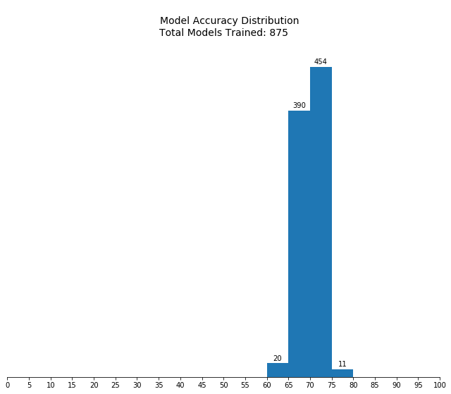
Fitting 5 folds for each of 175 candidates, totalling 875 fits


[Parallel(n_jobs=-1)]: Using backend LokyBackend with 12 concurrent workers.
[Parallel(n_jobs=-1)]: Done  17 tasks      | elapsed:    4.7s
[Parallel(n_jobs=-1)]: Done 138 tasks      | elapsed:   41.0s
[Parallel(n_jobs=-1)]: Done 341 tasks      | elapsed:  1.8min
[Parallel(n_jobs=-1)]: Done 624 tasks      | elapsed:  3.2min
[Parallel(n_jobs=-1)]: Done 875 out of 875 | elapsed:  4.5min finished
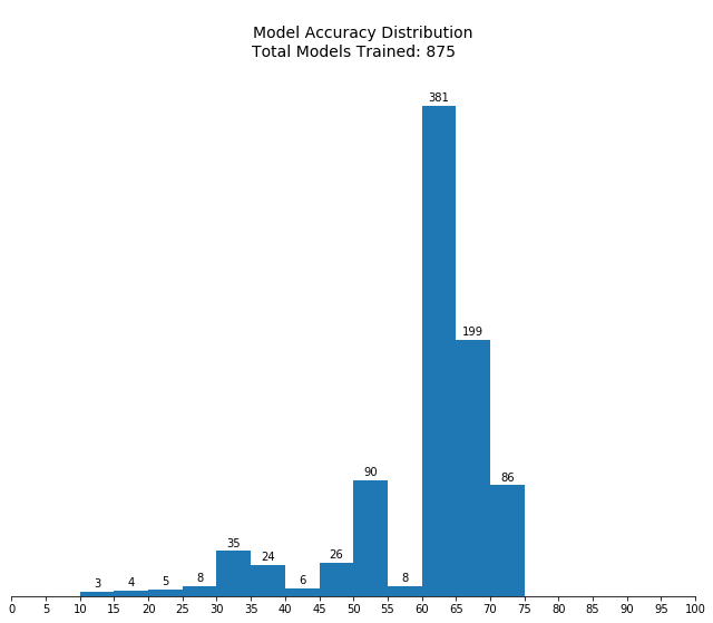
Notes from first pass:
- The top 10% of the configurations all had
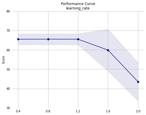
min_samples_leaf<= 0.1. - Mean performance drops and the standard deviation increases sharply with
learning_rate> 1.2.
clf = GradientBoostingClassifier(random_state=42)
parameters = {'learning_rate'     : np.arange( 0.2,  1.6,  0.2), # Default: 0.1
              'max_depth'         : np.arange(   1,    6,    1), # Default: 3
              'min_samples_leaf'  : np.arange(0.02, 0.12, 0.02)} # Default: 1

pass_2_r, pass_2_raw, pass_2_grid_fit = tune_and_visualize(clf, parameters)
Fitting 5 folds for each of 175 candidates, totalling 875 fits


[Parallel(n_jobs=-1)]: Using backend LokyBackend with 12 concurrent workers.
[Parallel(n_jobs=-1)]: Done  17 tasks      | elapsed:    4.3s
[Parallel(n_jobs=-1)]: Done 138 tasks      | elapsed:   58.9s
[Parallel(n_jobs=-1)]: Done 341 tasks      | elapsed:  2.5min
[Parallel(n_jobs=-1)]: Done 624 tasks      | elapsed:  4.7min
[Parallel(n_jobs=-1)]: Done 875 out of 875 | elapsed:  6.6min finished
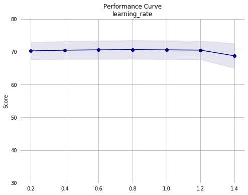
Notes from second pass:
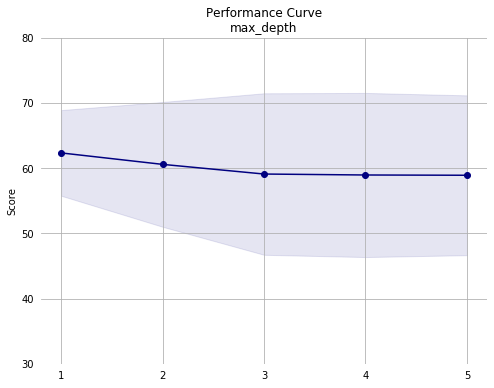
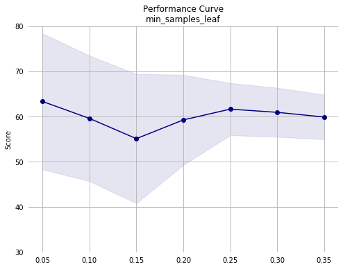
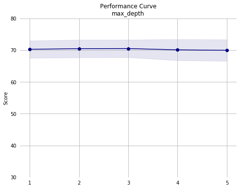
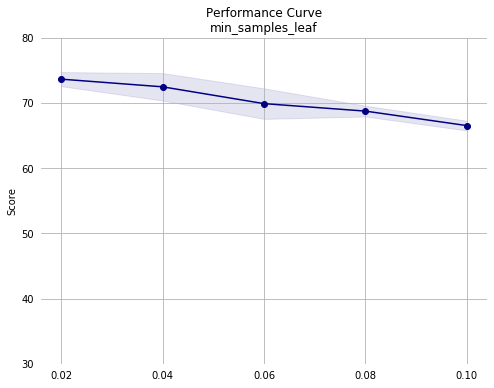
- Performance appears to decrease monotonically with increasing
min_samples_leaf. The training set consists of 36177 instances. Since we are using the default 5-fold validation, each model is trained on roughly 7235 instances. So, withmin_samples_leafof 0.02, each leaf must contain a minimum of roughly 145 instances. Given this, it may make sense to simply remove it as an optimization parameter since the default value is 1 node per leaf. - Performance across the other hyperparameters appears stable, except for a drop with
learning_rate> 1.2.
clf = GradientBoostingClassifier(random_state=42)
parameters = {'learning_rate'     : np.arange( 0.1,  1.3,  0.1), # Default: 0.1
              'max_depth'         : np.arange(   1,    6,    1), # Default: 3
              'min_samples_leaf'  : [1]}                         # Default: 1

pass_3_r, pass_3_raw, pass_3_grid_fit = tune_and_visualize(clf, parameters)
Fitting 5 folds for each of 60 candidates, totalling 300 fits


[Parallel(n_jobs=-1)]: Using backend LokyBackend with 12 concurrent workers.
[Parallel(n_jobs=-1)]: Done  17 tasks      | elapsed:   10.4s
[Parallel(n_jobs=-1)]: Done 138 tasks      | elapsed:  1.2min
[Parallel(n_jobs=-1)]: Done 300 out of 300 | elapsed:  2.6min finished
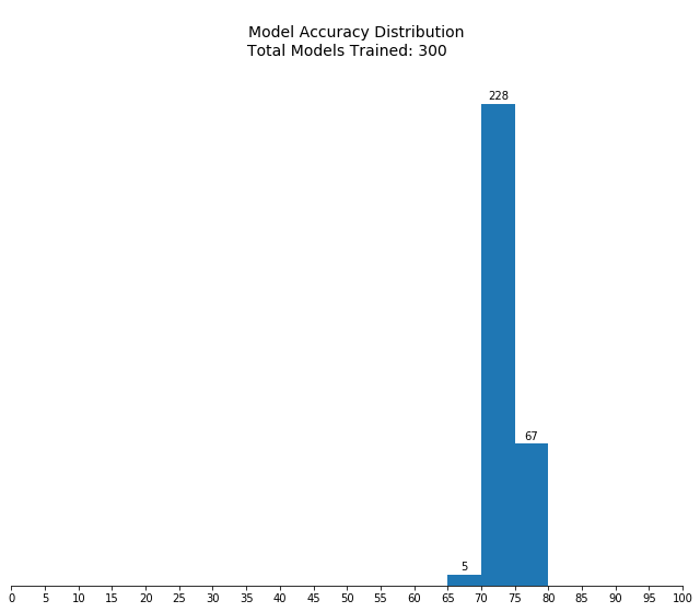
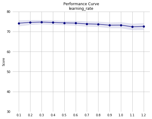
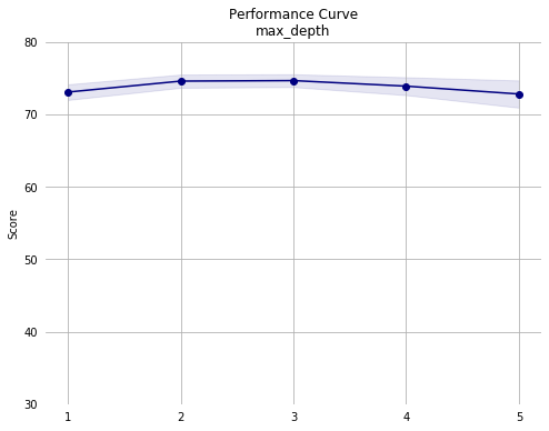
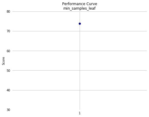
Notes from third pass:
- Mean performance appears fairly stable across hyperparameter ranges, indicating further optimization will yield diminishing returns.
Final Model Evaluation
from sklearn.metrics import (fbeta_score,
                             accuracy_score)
def plot_overlaid_performance_histograms(rs):
    plt.figure(figsize=(11,8.5))
    ax = plt.gca()

    for n, r in enumerate(rs):
        ax.hist(r['score'],
                bins=np.arange(0,105,5),
                alpha=0.35,
                align='mid',
                density=True,
                label='Pass ' + str(n+1))

    ax.set_xticks(np.arange(5,90,5))
    ax.set_xlim([5,85])

    ax.spines['left'].set_visible(False)
    ax.spines['top'].set_visible(False)
    ax.spines['right'].set_visible(False)

    plt.ylim([0,0.18])
    ymax = ax.get_ylim()[1]

    rects = ax.patches
    for n, rect in enumerate(rects):
        height = rect.get_height()
        if height > 0:
            # total area under each histogram with
            #      hist density parameter sums to 0.2.
            #      Factor of 5 corrects this.
            plt.gca().text(rect.get_x() + rect.get_width() / 2,
                           height + ymax/67,
                           '{}%'.format(int(round(height*100*5))),
                           ha='center',
                           va='center',
                           color=rect.get_facecolor(),
                           alpha=1)

    ax.set_xlabel('Score',
                  fontsize=12)
    ax.set_ylabel('% of Models Trained on that Pass',
                  fontsize=12)

    ax.tick_params(
        axis='y',
        left=False,
        labelleft=False)

    ax.legend(
    fancybox=True,
    loc=9,
    ncol=4,
    facecolor='white',
    edgecolor='white',
    framealpha=1,
    fontsize=12)

    ax.set_title('Performance Histograms by Grid Search Iteration',
                 fontsize=14)
plot_overlaid_performance_histograms([pass_1_r,
                                      pass_2_r,
                                      pass_3_r])
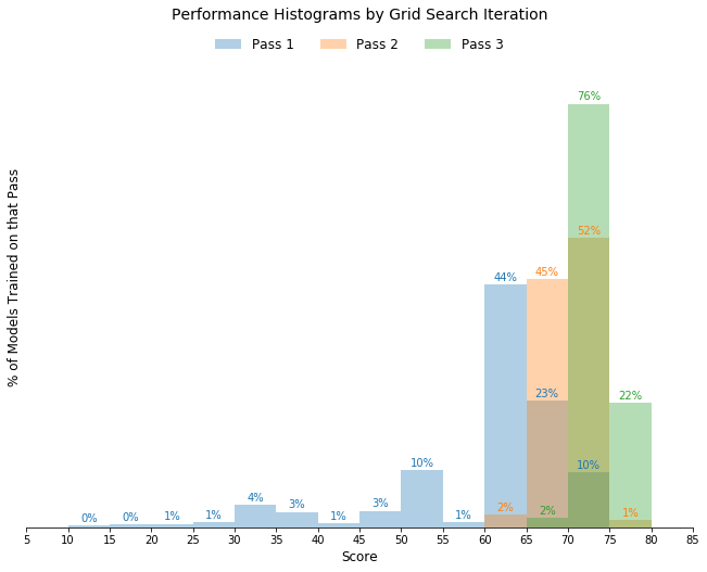
As shown in the overlaid histograms above, each successive grid search iteration resulted in improved performance distribution due to improved parameter search.
unoptimized = (GradientBoostingClassifier(random_state=42)
               .fit(X_train, y_train.values.ravel()))
unoptimized_preds = unoptimized.predict(X_test)
pass_1_preds = pass_1_grid_fit.best_estimator_.predict(X_test)
pass_2_preds = pass_2_grid_fit.best_estimator_.predict(X_test)
pass_3_preds = pass_3_grid_fit.best_estimator_.predict(X_test)

naive_pred_acc = 0.248
unoptimized_acc = accuracy_score(y_test, unoptimized_preds)
pass_1_acc = accuracy_score(y_test, pass_1_preds)
pass_2_acc = accuracy_score(y_test, pass_2_preds)
pass_3_acc = accuracy_score(y_test, pass_3_preds)

naive_pred_f_05 = 0.292
unoptimized_f_05 = fbeta_score(y_test, unoptimized_preds, beta = 0.5)
pass_1_f_05 = fbeta_score(y_test, pass_1_preds, beta = 0.5)
pass_2_f_05 = fbeta_score(y_test, pass_2_preds, beta = 0.5)
pass_3_f_05 = fbeta_score(y_test, pass_3_preds, beta = 0.5)
| Metric | Naive Predictor | Unoptimized Model | Pass 1 | Pass 2 | Pass 3 |
|---|---|---|---|---|---|
| Accuracy (%) | 24.8 | 86.3 | 85.1 | 86.4 | 87.1 |
| F-score (%) | 29.2 | 74.0 | 70.6 | 73.3 | 75.4 |
As shown in the scores calculated and then tabulated above, an unoptimized model is surprisingly good. The unoptimized model outperformed all models tuned during the Pass 1 and it outperformed all models in Pass 2 on F-score.
The best model constructed during Pass 3, however, outperformed the unoptimized model on both metrics.
Feature Importances
def feature_plot(importances, X_train, y_train):
    indices = np.argsort(importances)[::-1]
    columns = X_train.columns.values[indices[:5]]
    values = importances[indices][:5]

    # Creat the plot
    fig = plt.figure(figsize = (12,6))
    plt.title("Normalized Weights for First Five Most Predictive Features", fontsize = 16)
    plt.bar(np.arange(5), values, width = 0.6, align="center",
            label = "Feature Weight")
    plt.bar(np.arange(5) - 0.3, np.cumsum(values), width = 0.2, align = "center",
            label = "Cumulative Feature Weight")

    plt.xticks(np.arange(5), columns)
    plt.xlim((-0.5, 4.5))
    plt.ylim([0,1])

    plt.ylabel("Weight", fontsize = 12)
    plt.xlabel("Feature", fontsize = 12)

    plt.legend(
    fancybox=True,
    loc=9,
    ncol=4,
    facecolor='white',
    edgecolor='white',
    framealpha=1,
    fontsize=12)

    for spine in plt.gca().spines.values():
        spine.set_visible(False);

    plt.tick_params(
        axis='x',
        bottom=False)
    plt.tick_params(
        axis='y',
        left=False,
        right=False,
        labelleft=False)

    rects = plt.gca().patches
    for n, r in enumerate(rects):
        height = r.get_height()
        plt.gca().text(r.get_x() + r.get_width() / 2,
                       height+.025,
                       '{:1.2f}'.format(height),
                       ha='center',
                       va='center')

    plt.tight_layout()
importances = pass_3_grid_fit.best_estimator_.feature_importances_
feature_plot(importances, X_train, y_train)
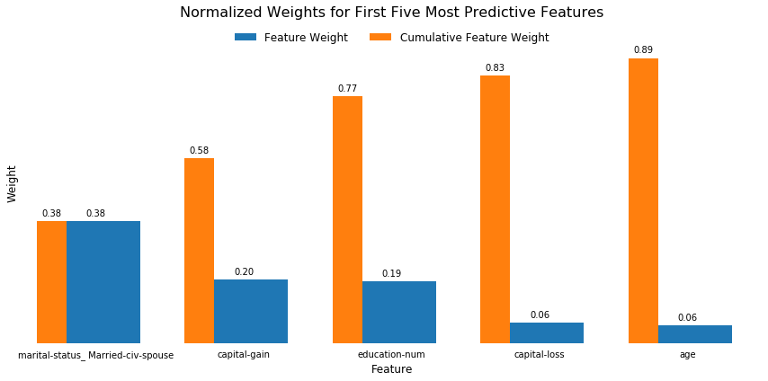
Some of the most important features are intuitive. Others are not.
- I expect that people who are financially sophisticated enough to report their capital gains and capital losses would also have relatively high earning potential.
- I would also expect that more educated and older individuals to have increased earning potential.
- It is surprising to me that being married is the most important factor. I would have expected it to be important, but less important than the other factors in the top 5.
Feature Selection
The top-five most important features are shown in the graph above and listed below.
marital-status_Married-civ-spouse- Binary, whether individual is married and civil with their spouse.capital-gain- Continuous, how much capital gain the individual reported.education-num- Categorical, a proxy for how well-educated the person is.capital-loss- Continuous, how much capital loss the individual reported.age- Discrete, how old the individual is.
from sklearn.base import clone

X_train_reduced = X_train[X_train.columns.values[(np.argsort(importances)[::-1])[:5]]]
X_test_reduced = X_test[X_test.columns.values[(np.argsort(importances)[::-1])[:5]]]

reduced_clf = ((clone(pass_3_grid_fit.best_estimator_))
               .fit(X_train_reduced, y_train.values.ravel()))

reduced_predictions = reduced_clf.predict(X_test_reduced)

reduced_acc = accuracy_score(y_test, reduced_predictions)
reduced_f_05 = fbeta_score(y_test, reduced_predictions, beta = 0.5)
| Metric | Naive Predictor | Unoptimized Model | Pass 1 | Pass 2 | Pass 3 | Pass 3 Reduced Data |
|---|---|---|---|---|---|---|
| Accuracy (%) | 24.8 | 86.3 | 85.1 | 86.4 | 87.1 | 85.9 |
| F-score (%) | 29.2 | 74.0 | 70.6 | 73.3 | 75.4 | 72.8 |
The fully-optimized model performs slightly worse when trained on only the top five features tabulated above. Notably, it does perform worse than an unoptimized model trained on all the data, however. In this situation, training is not time- or resource-prohibitive, so there is not much sense in limiting the feature space to anything less than the full dataset.
I can imagine situations where this is not the case, however, and it is necessary to reduce the dimensionality of the training data even if there is a small negative impact to overall model performance.