Optimizing a Classifier for Profitability
The goal of this short analysis project is to create a predictive model to determine which future credit card applicants should be approved or rejected for a credit card. The model is designed to maximize total bank profits.
Stated more precisely, the goal is to create a binary classification scheme that selects customers that are most likely to be profitable for the bank. Note that the set of profitable customers is not identical to the set of customers who do not default.
The Data
The data utilized consists of two sets of 200 customers, their creditworthiness metrics, and profitability outcomes.
The first five rows of the training data are shown below.
| Age | Years at Employer | Years at Address | Income | Credit Card Debt | Automobile Debt | Net Profits |
|---|---|---|---|---|---|---|
| 32.53 | 9.39 | 0.30 | $37,844 | ($3,247) | ($4,795) | $3,206 |
| 34.58 | 11.97 | 1.49 | $65,765 | ($15,598) | ($17,632) | $2,940 |
| 37.70 | 12.46 | 0.09 | $61,002 | ($11,402) | ($7,910) | ($1,024) |
| 28.68 | 1.39 | 1.84 | $19,953 | ($1,233) | ($2,408) | $2,945 |
| 32.61 | 7.49 | 0.23 | $24,970 | ($1,136) | ($397) | $738 |
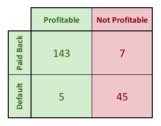
At left I show a matrix of which applicant profitability and whether they paid off their card. There is significant overlap between the set of applicants who paid off their card and who were profitable for the bank, but there is not perfect correspondence. In particular, people who manage their credit extremely carefully and rarely incur any sort of financial fees may cost the bank more in administrative overhead than they make the bank in fees.
Model Creation Plan
In a binary classification system with binary outcomes, the objective is to maximize the Area under the Curve (AUC), where the “curve” is the receiver operating characteristic (ROC) curve. Generating this curve is accomplished by rank-ordering the data according to a model, and generating a plot of the “False Positive Rate” (X) versus the “True Positive Rate” (Y) for all possible model thresholds. Developing this plot requires labeled training data with known outcomes. The model is fine-tuned in order to maximize the area under the curve, thereby increasing the model’s predictive power. Finally, selecting the optimal threshold is a matter of assigning costs to false positives and false negatives. The threshold that minimizes the resulting weighted sum of products is the appropriate one to select.
Analogous Process for Non-Binary Dependent Variables
In this case, the outcomes are not binary, but weighted. The most profitable applicants the bank obtains can be worth many thousands of dollars. For the training data, the top three most profitable customers can be worth many thousands of dollars (top three: $35,096, $23,910, and $18,807). The least profitable customers cost the bank decidedly less (bottom three: -$8,343, -$8,669, and -$9,142). This is obviously a very different exercise than binary classification.
But, an analogous process can be applied. The optimization process will involve multiple linear regression using the training data to determine the optimal coefficients for each of the six standardized, independent variables. This regression line will create an expected profitability for each applicant. The applicants will be rank-ordered using this expected profitability, and a running sum of the actual profitability (starting from the highest expected value customer) will be calculated. The cutoff (or “threshold”) that maximizes the total revenue for the bank will be selected.
Creating the Model
First, I generate the standard deviation and mean for the training data.
| Age | Years at Employer | Years at Address | Income | Credit Card Debt | Automobile Debt | Profit | |
|---|---|---|---|---|---|---|---|
| Mean | 34.67 | 8.61 | 0.78 | 48439.96 | -3202.11 | -6378.07 | 1905.51 |
| Std Dev | 8.20 | 6.77 | 0.62 | 47862.35 | 3892.03 | 7472.44 | 5755.91 |
Then, I standardize the data.
| Age | Years at Employer | Years at Address | Income | Credit Card Debt | Automobile Debt | Profit |
|---|---|---|---|---|---|---|
| -0.26 | 0.11 | -0.78 | -0.22 | -0.01 | 0.21 | 0.23 |
| -0.01 | 0.50 | 1.14 | 0.36 | -3.18 | -1.51 | 0.18 |
| 0.37 | 0.57 | -1.12 | 0.26 | -2.11 | -0.21 | -0.51 |
| -0.73 | -1.07 | 1.71 | -0.60 | 0.51 | 0.53 | 0.18 |
| -0.25 | -0.17 | -0.88 | -0.49 | 0.53 | 0.80 | -0.20 |
Using Excel’s LINEST, I generate the following coefficients and data. Recall that the first line are the $\beta$s, or coefficients.
| Auto Debt | CC Debt | Income | YAA | YAE | Age | |
|---|---|---|---|---|---|---|
| -0.005 | -0.055 | 0.639 | -0.066 | 0.187 | 0.008 | 0.000 |
| 0.058 | 0.062 | 0.073 | 0.043 | 0.058 | 0.051 | 0.042 |
| 0.655 | 0.598 | #N/A | #N/A | #N/A | #N/A | #N/A |
| 61.2 | 193 | #N/A | #N/A | #N/A | #N/A | #N/A |
| 131.1 | 68.9 | #N/A | #N/A | #N/A | #N/A | #N/A |
Using these regression coefficients, the MLR model becomes the following.
$$\text{Profit/Loss} = -0.005(\text{Auto Debt}) - 0.055(\text{CC Debt}) + $$
$$0.639(\text{Income}) - 0.066(\text{Years at Add}) + $$
$$0.187(\text{Years at Emp}) + 0.008(\text{Age})$$
Using that model, I generate values for expected profits in terms of z-score. Using the average and standard deviation for the actual profits, I calculated expected profits in terms of dollars.
| ID | Exp Profits (z) | Exp Profits ($) | Act Profits ($) |
|---|---|---|---|
| 1 | -0.07 | $1,494 | $3,206 |
| 2 | 0.43 | $4,390 | $2,940 |
| 3 | 0.47 | $4,600 | $(1,024) |
| 4 | -0.73 | $(2,292) | $2,945 |
| 5 | -0.32 | $54 | $738 |
Next, I rank order the applicants in terms of Expected Profits. I also create a running cumulative sum of actual profits divided by total applicants. Those values are the actual average profits per applicant, if the profitability threshold is set just below that particular applicant’s expected profits.
| ID | Exp Profits (z) | Exp Profits ($) | Act Profits ($) | Act Profits/App at Threshold ($) |
|---|---|---|---|---|
| 51 | 6.09 | $36,930 | $35,096 | $175 |
| 81 | 3.58 | $22,501 | $23,910 | $295 |
| 100 | 3.47 | $21,882 | $18,807 | $389 |
| 6 | 2.30 | $15,132 | $16,969 | $474 |
| 15 | 2.10 | $13,971 | $11,754 | $533 |
I search the actual average profits/applicant column for the maximum value. The neighborhood surrounding that maximum value is shown below.
| ID | Exp Profits (z) | Exp Profits ($) | Act Profits ($) | Act Profits/App at Threshold ($) | |
|---|---|---|---|---|---|
| 160 | -0.31 | $102 | $932 | $2,461 | |
| 69 | -0.32 | $88 | $1,615 | $2,470 | |
| 134 | -0.32 | $88 | $3,375 | $2,486 | « |
| 73 | -0.32 | $71 | $(8,101) | $2,446 | |
| 5 | -0.32 | $54 | $738 | $2,450 |
The threshold needs to be set at a z-value between -0.318 and -0.316. -0.317 will work.
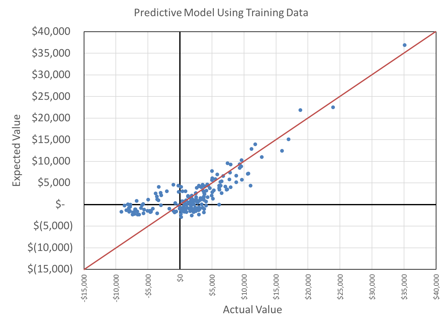
The following plots of actual profits versus expected profits, and the histogram of actual profits, are not used to analyze the model in a rigorous fashion but they are informative.
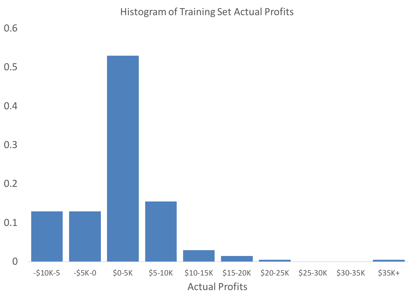
As is obvious from the probability histogram below, the data exhibits significant skew.
Example Applicant
An example applicant might have the following z-scores.
| Age | Years at Emp | Years at Address | Income | Credit Card Debt | Auto Debt |
|---|---|---|---|---|---|
| -0.06 | 0.23 | -0.58 | -0.38 | 0.14 | -0.06 |
Applying the model results in an aggregate z-score of -0.170. Since this applicant is above the threshold value of -0.317, s/he would be approved.
Performance Testing on Training Set
Average Profit per Applicant
There are two “bounding values” for the average profit per applicant metric that are worthy of discussion. An ideal (and impossible?) model that only approved applicants that were profitable for the bank would have produced a total profit of $631,777, or roughly $3,158 per applicant. Simply approving all applicants would have produced a total profit of $381,103, or $1,906 per applicant.
Applying the model to the training set results in an average per-applicant profit of $2,486. This value is taken from the rank-order table listed above. It is calculated as the sum of all the profits (and losses) of the applicants with z-scores greater than the threshold value of -0.317.
Incremental Profit per Applicant
The incremental value per applicant over simply approving all applicants is calculated as follows.
$$$2486-$1906=$580$$
$$\frac{$580}{$1906}=30%$$
Expressed as a percentage, this is a 30% increase over the baseline.
Performance Testing on Test Set
As expected, applying this model to the test set data produces a worse correlation. This can be noted visually in the following scatterplot.
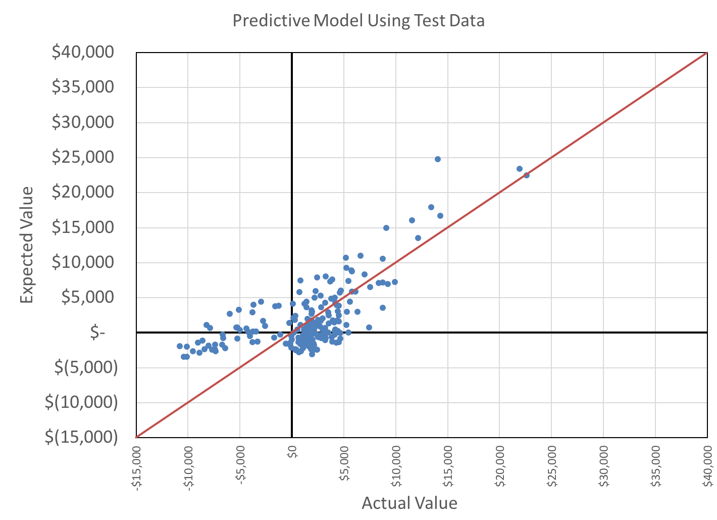
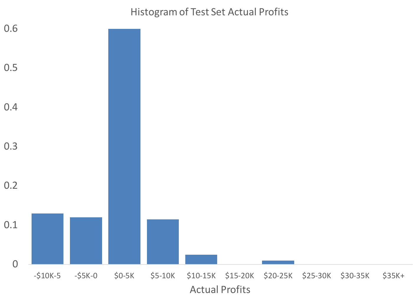
I perform a sanity-check on the data to ensure the actual profits are distributed roughly the same as the training data. The axes are fixed to the same values as the training set histogram, above, for easy visual comparison.
The distributions are roughly similar, although I note that the test set seems to exhibit less skew. And, the positive side datapoint in the training data may constitute an outlier.
Average Profit per Applicant
As with the training data, I compute the bounding values for the average profit per applicant metric. For this dataset, a perfect model would have resulted in a total profit of $554,797 or $2,774 per applicant. Simply approving all the application would have resulted in total profits of $306,528 or $1,533 per applicant.
Applying the model to the test set results in an average per-applicant profit of $1,771. Again, this value is calculated as the sum of all the profits (and losses) of the applicants with z-scores greater than the threshold value of -0.317.
Incremental Profit per Applicant
These calculations are performed similarly to those for the training set data. The percentage increase over baseline is slightly less than that for the training data, at 16%.
$$$1771-$1533=$238$$
$$\frac{$238}{$1533}=16%$$
Check for Overfitting
In order to check for model overfitting, the standard deviations of model errors are calculated for training and test data. The model error, or the “residuals,” are calculated as
$$profits_{expected}-profits_{actual}$$
The standard deviation of errors are represented as $\sigma_e$. The ratio is as follows.
$$\frac{\sigma_{e,test}}{\sigma_{e,training}}=\frac{3867}{3379}=14%$$
The benchmark for overfitting is that the standard deviation of model error must increase by less than 20% between the test and training data. In this case, it does, which suggests I can have very high confidence of minimal over-fitting.
Data_Final-Project.xlsx
Some other content is taken from my notes on other aspects of the aforementioned Coursera course.