Using PCA on Cars Dataset
import pandas as pd
import numpy as np
from sklearn.decomposition import PCA
from sklearn.preprocessing import StandardScaler

import matplotlib.pyplot as plt
The dataset for this example consists of 387 cars with 18 features. 7 of these features are dummy variables.
c = pd.read_csv('pca-on-cars-dataset/cars.csv')
c.info()
c.head().T
<class 'pandas.core.frame.DataFrame'>
Index: 387 entries, Acura 3.5 RL to Volvo XC90 T6
Data columns (total 18 columns):
 #   Column      Non-Null Count  Dtype
---  ------      --------------  -----
 0   Sports      387 non-null    int64
 1   SUV         387 non-null    int64
 2   Wagon       387 non-null    int64
 3   Minivan     387 non-null    int64
 4   Pickup      387 non-null    int64
 5   AWD         387 non-null    int64
 6   RWD         387 non-null    int64
 7   Retail      387 non-null    int64
 8   Dealer      387 non-null    int64
 9   Engine      387 non-null    float64
 10  Cylinders   387 non-null    int64
 11  Horsepower  387 non-null    int64
 12  CityMPG     387 non-null    int64
 13  HighwayMPG  387 non-null    int64
 14  Weight      387 non-null    int64
 15  Wheelbase   387 non-null    int64
 16  Length      387 non-null    int64
 17  Width       387 non-null    int64
dtypes: float64(1), int64(17)
memory usage: 57.4+ KB
| Acura 3.5 RL | Acura 3.5 RL Navigation | Acura MDX | Acura NSX S | Acura RSX | |
|---|---|---|---|---|---|
| Sports | 0.0 | 0.0 | 0.0 | 1.0 | 0.0 |
| SUV | 0.0 | 0.0 | 1.0 | 0.0 | 0.0 |
| Wagon | 0.0 | 0.0 | 0.0 | 0.0 | 0.0 |
| Minivan | 0.0 | 0.0 | 0.0 | 0.0 | 0.0 |
| Pickup | 0.0 | 0.0 | 0.0 | 0.0 | 0.0 |
| AWD | 0.0 | 0.0 | 1.0 | 0.0 | 0.0 |
| RWD | 0.0 | 0.0 | 0.0 | 1.0 | 0.0 |
| Retail | 43755.0 | 46100.0 | 36945.0 | 89765.0 | 23820.0 |
| Dealer | 39014.0 | 41100.0 | 33337.0 | 79978.0 | 21761.0 |
| Engine | 3.5 | 3.5 | 3.5 | 3.2 | 2.0 |
| Cylinders | 6.0 | 6.0 | 6.0 | 6.0 | 4.0 |
| Horsepower | 225.0 | 225.0 | 265.0 | 290.0 | 200.0 |
| CityMPG | 18.0 | 18.0 | 17.0 | 17.0 | 24.0 |
| HighwayMPG | 24.0 | 24.0 | 23.0 | 24.0 | 31.0 |
| Weight | 3880.0 | 3893.0 | 4451.0 | 3153.0 | 2778.0 |
| Wheelbase | 115.0 | 115.0 | 106.0 | 100.0 | 101.0 |
| Length | 197.0 | 197.0 | 189.0 | 174.0 | 172.0 |
| Width | 72.0 | 72.0 | 77.0 | 71.0 | 68.0 |
Helper function that performs the scaling and actual PCA.
def do_pca(n_components, data):
    X = StandardScaler().fit_transform(data)
    pca = PCA(n_components)
    X_pca = pca.fit_transform(X)

    return pca, X_pca
Helper function that:
- Creates a DataFrame of the PCA results
- Includes feature weights and explained variance
- Visualizes the PCA results
def pca_results(full_dataset, pca, plot=True):
    '''
    Create a DataFrame of the PCA results
    Includes dimension feature weights and explained variance
    Visualizes the PCA results
    '''

    # Dimension indexing
    dimensions = dimensions = \
    ['Dimension {}'.format(i) for i in range(1,len(pca.components_)+1)]

    # PCA components
    components = pd.DataFrame(np.round(pca.components_, 4), columns = full_dataset.keys())
    components.index = dimensions

    # PCA explained variance
    ratios = pca.explained_variance_ratio_.reshape(len(pca.components_), 1)
    variance_ratios = pd.DataFrame(np.round(ratios, 4), columns = ['Explained Variance'])
    variance_ratios.index = dimensions

    if plot:
        # Create a bar plot visualization
        fig, ax = plt.subplots(figsize = (14,8))

        # Plot the feature weights as a function of the components
        components.plot(ax = ax, kind = 'bar');
        ax.set_ylabel("Feature Weights")
        ax.set_xticklabels(dimensions, rotation=0)

        # Display the explained variance ratios
        for i, ev in enumerate(pca.explained_variance_ratio_):
            ax.text(i-0.40, ax.get_ylim()[1] + 0.05,
                    "Explained Variance\n          %.4f"%(ev))

    # Return a concatenated DataFrame
    return pd.concat([variance_ratios, components], axis = 1)
For context, as outlined in my other notes on PCA:
- Principal components span the directions of maximum variability.
- Principal components are always orthogonal to one another.
- Eigenvalues tell us the amount of information a principal component holds.
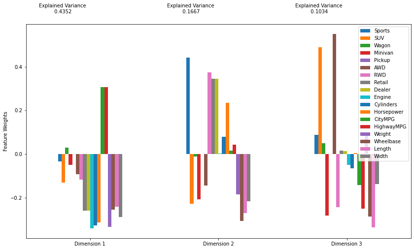
First, consider the first 3 principal components:
pca, X_pca = do_pca(3, c)
pca_results(c, pca).T
| Dimension 1 | Dimension 2 | Dimension 3 | |
|---|---|---|---|
| Explained Variance | 0.4352 | 0.1667 | 0.1034 |
| Sports | -0.0343 | 0.4420 | 0.0875 |
| SUV | -0.1298 | -0.2261 | 0.4898 |
| Wagon | 0.0289 | -0.0106 | 0.0496 |
| Minivan | -0.0481 | -0.2074 | -0.2818 |
| Pickup | 0.0000 | -0.0000 | 0.0000 |
| AWD | -0.0928 | -0.1447 | 0.5506 |
| RWD | -0.1175 | 0.3751 | -0.2416 |
| Retail | -0.2592 | 0.3447 | 0.0154 |
| Dealer | -0.2576 | 0.3453 | 0.0132 |
| Engine | -0.3396 | 0.0022 | -0.0489 |
| Cylinders | -0.3263 | 0.0799 | -0.0648 |
| Horsepower | -0.3118 | 0.2342 | 0.0040 |
| CityMPG | 0.3063 | 0.0169 | -0.1421 |
| HighwayMPG | 0.3061 | 0.0433 | -0.2486 |
| Weight | -0.3317 | -0.1832 | 0.0851 |
| Wheelbase | -0.2546 | -0.3066 | -0.2846 |
| Length | -0.2414 | -0.2701 | -0.3361 |
| Width | -0.2886 | -0.2163 | -0.1369 |
print('Number of Components :   Variance Explained')
for component_count in range(1,17):
    pca, X_pca = do_pca(component_count, c)
    results = pca_results(c, pca, False)
    print('{:20} :   {:2.1%}'.format(component_count,
                                     results['Explained Variance'].sum()))
Number of Components :   Variance Explained
                   1 :   43.5%
                   2 :   60.2%
                   3 :   70.5%
                   4 :   76.8%
                   5 :   82.4%
                   6 :   86.8%
                   7 :   89.7%
                   8 :   92.5%
                   9 :   95.0%
                  10 :   96.8%
                  11 :   97.7%
                  12 :   98.5%
                  13 :   99.0%
                  14 :   99.5%
                  15 :   99.8%
                  16 :   100.0%
Note that the first two components, alone, account for 60% of the variance in the dataset.
This content is taken from notes I took while pursuing the Intro to Machine Learning with Pytorch nanodegree certification.