Gaussian Mixture Models and Cluster Validation

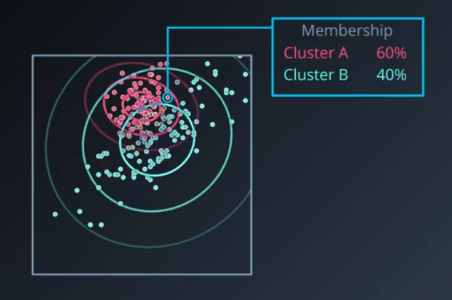
Gaussian Mixture Model Clustering is a “soft” clustering algorithm that means every sample in our dataset will belong to every cluster that we have, but will have different levels of membership in each cluster.

The algorithm works by grouping points into groups that seem to have been generated by a Gaussian distribution.

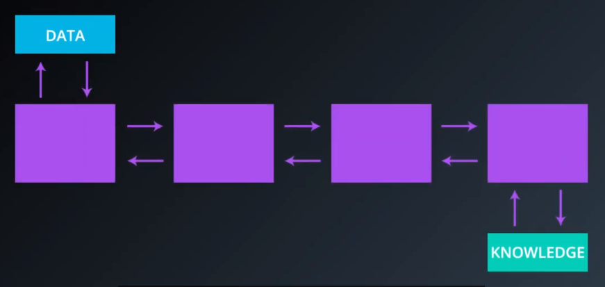
The Cluster Analysis Process is a means of converting data into knowledge and requires a series of steps beyond simply selecting an algorithm. This page overviews that process.

Cluster Validation is the process by which clusterings are scored after they are executed. This provides a means of comparing different clustering algorithms and their results on a certain dataset.

Gaussian Mixture Modeling

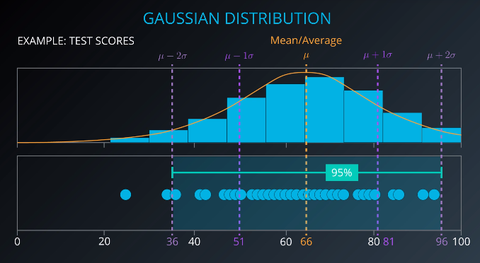
Gaussian Mixture Modeling is probably the most advanced clustering method overviewed as part of the nanodegree. It assumes that each cluster follows a normal distribution.

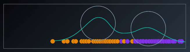
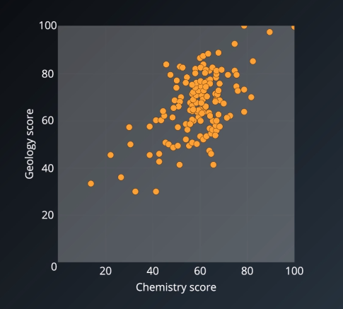
The dataset shown below contains the superposition of two Gaussians clusters, which the Gaussian mixture model would tease apart. Whichever point seems to have the highest probabiltiy to have come from each Gaussian is classified as belonging to a separate cluster.

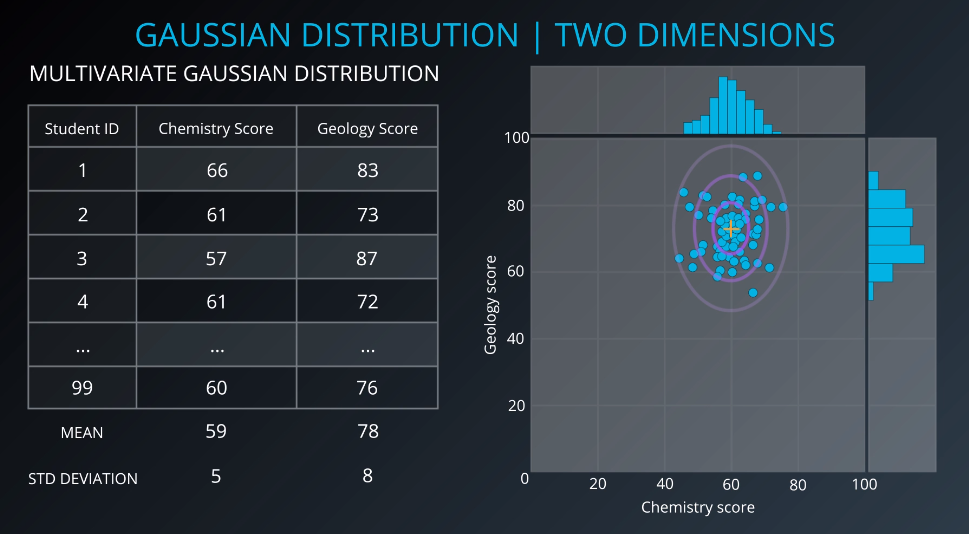
Consider a dataset containing a chemistry test score and a geology test score for each of 99 students. Since this dataset has more than one variable and each of the two variables is a Gaussian distribution, this dataset is called a multivariate Gaussian distribution. So, it is a Gaussian distribution in more than one variable.

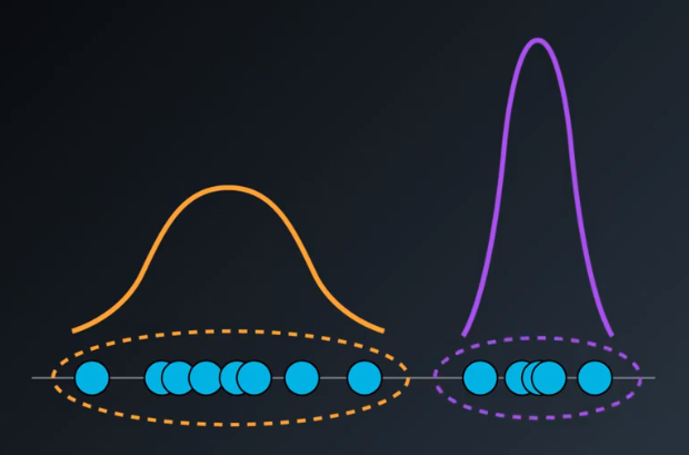
Consider a situation where we have similar Gaussian distributions for each of two cohorts of students.

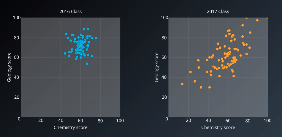
Then, consider that we mixed the two datasets together and accidentally remove the labels. The resulting composite dataset would not be Gaussian, but we would know it is composed of two Gaussian distributions. This would be an appropriate conditions for us to do Gaussian mixture modeling to try to retrieve the original distributions.

Gaussian Mixture Model Clustering Algorithm

This is called the “Expectation-Maximization algorithm for Gaussian mixtures”

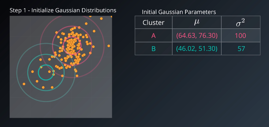
1. Initialize K Gaussian Distributions (for example posed above, k=2)
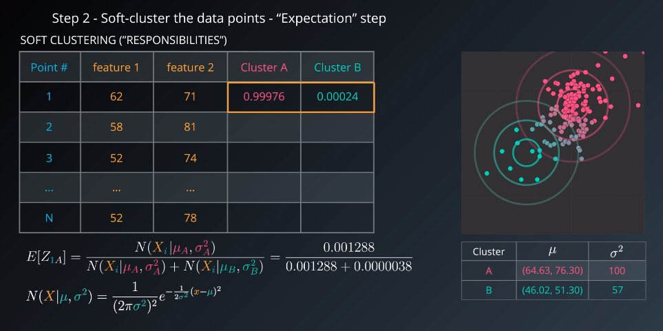
2. Soft-cluster data (called “expectation” step)
3. Re-estimate the Gaussians (called “maximization” step)
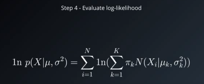
4. Evaluate the log-likelihood to check for convergence. Repeat from Step #2 until converged.

Step 1

Step 2

Step 3

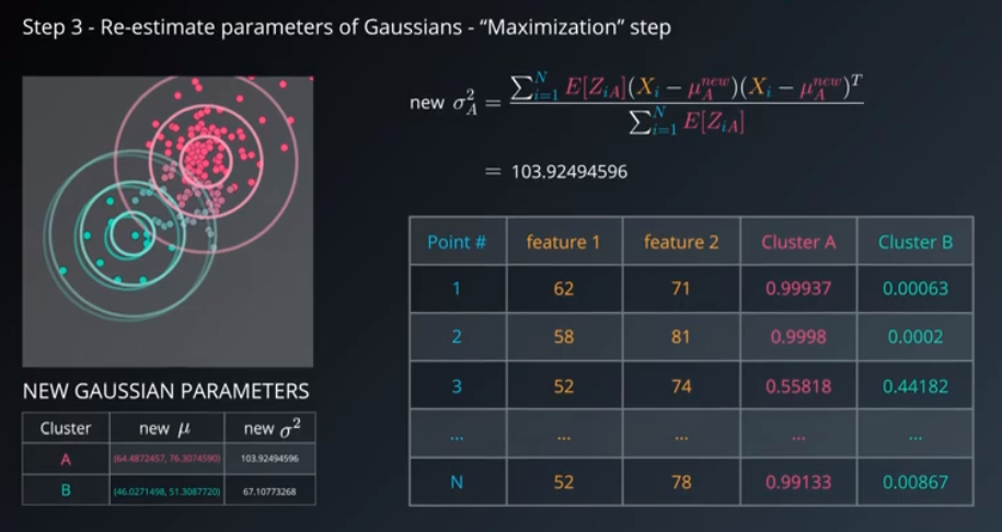
Step 4

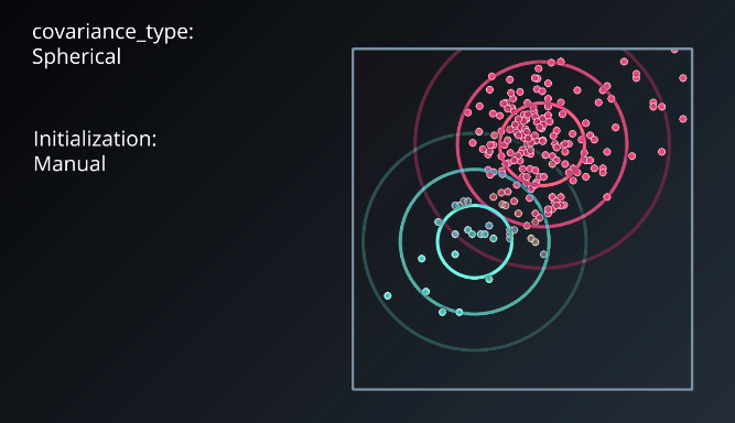
The results of running the algorithm are shown below. These clusters do not resemble the initial datasets that were mixed. This is due to using covariance_type: “spherical” and initialization: “manual”.

If, instead, we use covariance_type: “full” and the initialization: “default (k-means)” we get something much closer to the original datasets.

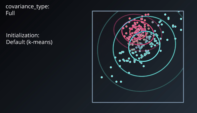
This example shows how important it is to be careful when choosing the parameters of the initial Gaussians. It has s significant effect on the quality of the algorithm’s result.

Gaussian Mixture Models Examples and Applications

Advantages:

• Soft-clustering (sample membership of multiple clusters)
• Cluster shape flexibility

Disadvantages:

• Sensitive to initialization values
• Possible to converge to a local optimum
• Slow convergence rate

Several examples for Gaussian Mixuture modeling are linked below.

• Nonparametric discovery of human routines from sensor data
• Application of the Gaussian mixture model in pulsar astronomy
• Speaker Verification Using Adapted Gaussian Mixture Models
• Adaptive background mixture models for real-time tracking
• Background image subtraction from Video

Cluster Analysis

There are several steps involved in converting a dataset into knowledge and information.

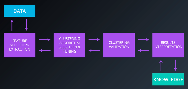
1. Feature Selection: Choosing distinguishing features from a set of candidates. Datasets can have thousands of dimensions.
   Feature Extraction: Transforming the data to generate novel and useful features. The best example of this is PCA (principle component analysis).
2. Clustering Algorithm Selection: No algorithm is universally applicable and experimentation is often required.
   Proximity Measure Selection: Examples so far have used Euclidean distance. If the data is documents or word embeddings, the proximity measure will be cosine distance. If it is gene expression, it might be Pearson’s correlation.
3. Clustering Validation: Evaluating how well a clustering exercise went via visualization or scoring methods. The scoring methods are called indices, and each of them is called a clustering validation index.
4. Results Interpretation: Determining what insights we can glean from the resulting clustering structure. This step requires domain expertise to give labels to the clusters and infer insights from them.

Cluster Validation

Cluster validation is the procedure for evaluating the results of a clustering objectively and quantitatively. There are three categories of cluster validation indices:

1. External indices: Used if the data was originally labeled.
2. Internal indices: Used if the data was not labeled (commonly the case for unsupervised learning). These measure the fit between the data and the structure using only the data.
3. Relative indices: Indicate which of two clustering structures is better in some sense. All internal indices can serve as relative indices.

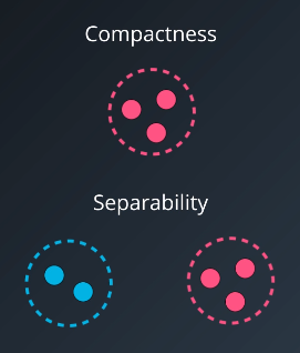
Most validation indices are defined by combining compactness and separability. Compactness is a measure of how close the elements of a cluster are to each other. Separability is a measure of how far or distinct clusters are from each other.

External Indices

External validation indices are used when we have a labeled dataset.

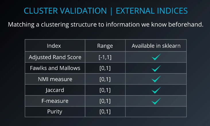
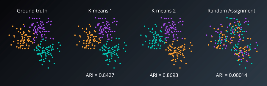
For example, a higher adjusted rand index indicates a better fit with the ground truth.

The adjusted rand index does not care if the actual labels match. It only cares that the points that were in a cluster in the ground together remain in a cluster in the clustering result, regardless of whether the clustering algorithm gives the cluster the label ‘0’ or ‘1’.

Internal Indices

Internal validation indices are can be used for non-labeled datasets.

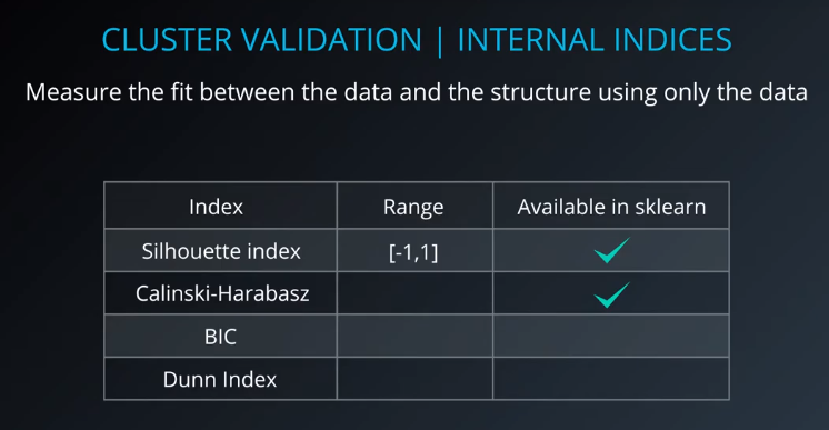
The Silhouette coefficient is a value between -1 and 1, where higher values indicate a better clustering. This index is especially useful for high-dimensional datasets where visualizing the clusterings is not possible. We can also calculate the silhouette coefficient for each point; values for individual points are calcualted by averaging across clusters or an entire dataset.

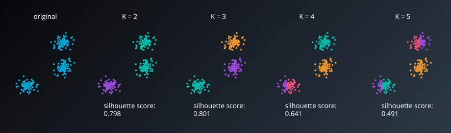
As shown below, increasing $K$ dramatically does not result in a higher score.

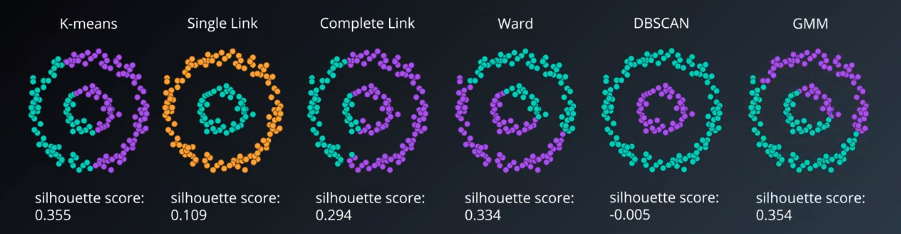
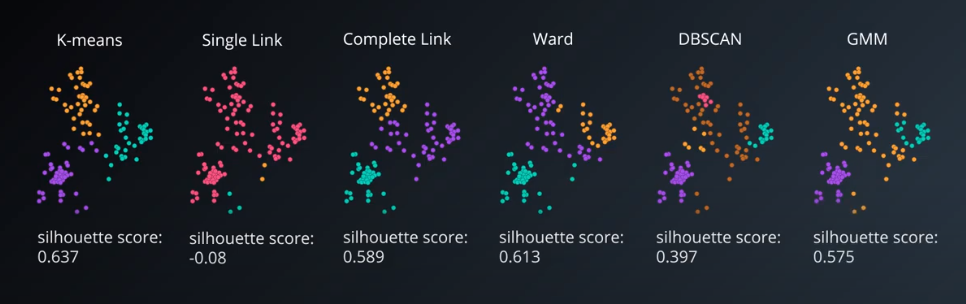
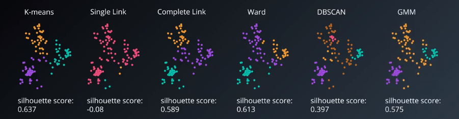
The Silhouette coefficient can also be used to compare clustering algorithms and how they did on a certain dataset. If multiple algorithms produce the same clustering they get the same result.

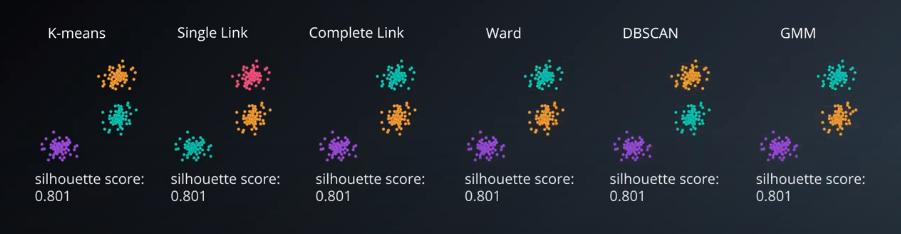
Note that Silhouette coefficient is not a good index for DBSCAN because Silhouette does not have the concept of noise and DBSCAN tends not to have the compact clusters that Silhouette rewards. An algorithm like DBCV (Density-Based Clustering Validation) would be much better for DBSCAN.

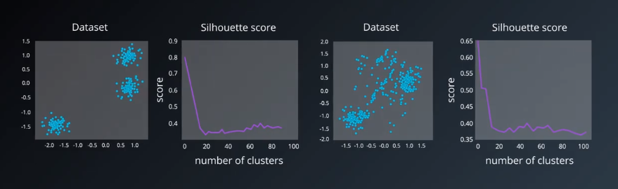
The example below shows a downside of Silhouette. If we compare Silhouette values on the two rings dataset we see that it is not built to reward carving out complex clusters like this. Silhouette is built to find well-separated, dense, circular clusters.