Dimensionality Reduction and PCA

PCA, or Principle Component Analysis, is a means of reducing the dimensionality of datasets. It is an example of transforming not clustering it, like the other notes so far in this section. Dimensionality Reduction means taking a full dataset and reducing it to just the features that contain the most information.

Latent Features

With large datasets we often suffer with what is known as the “curse of dimensionality,” and need to reduce the number of features to effectively develop a model. Feature Selection and Feature Extraction are two general approaches for reducing dimensionality.

Principal Component Analysis is a common method for extracting new “latent features” from our dataset, based on existing features. Latent Features are features that aren’t explicitly in the dataset. They are not directly observed, but underlie other features that are observed.

Consider an example of a set of features from common questions on company surveys:

1. I feel that my manager is supportive of my growth within the company.
2. I feel confident that I can contribute to the company goals.
3. I feel that my work contributes positively to the world.
4. I feel that my opinions are heard when making decisions about company decisions.
5. My peers are supportive of my contributions.

These questions could be reasonably grouped into the two latent features shown below.

Supportive Work Environment: 1, 4, 5
Confidence to Make an Impact: 2, 3

Consider another dataset that contains the following features related to homes:

• lot size
• number of rooms
• floor plan size
• size of garage
• number of bedrooms
• number of bathrooms
• local crime rate
• number of schools in five miles
• property tax rate
• local median income
• average air quality index
• distance to highway

These features can be logically grouped into two broad categories: the size of the house and the neighborhood quality.

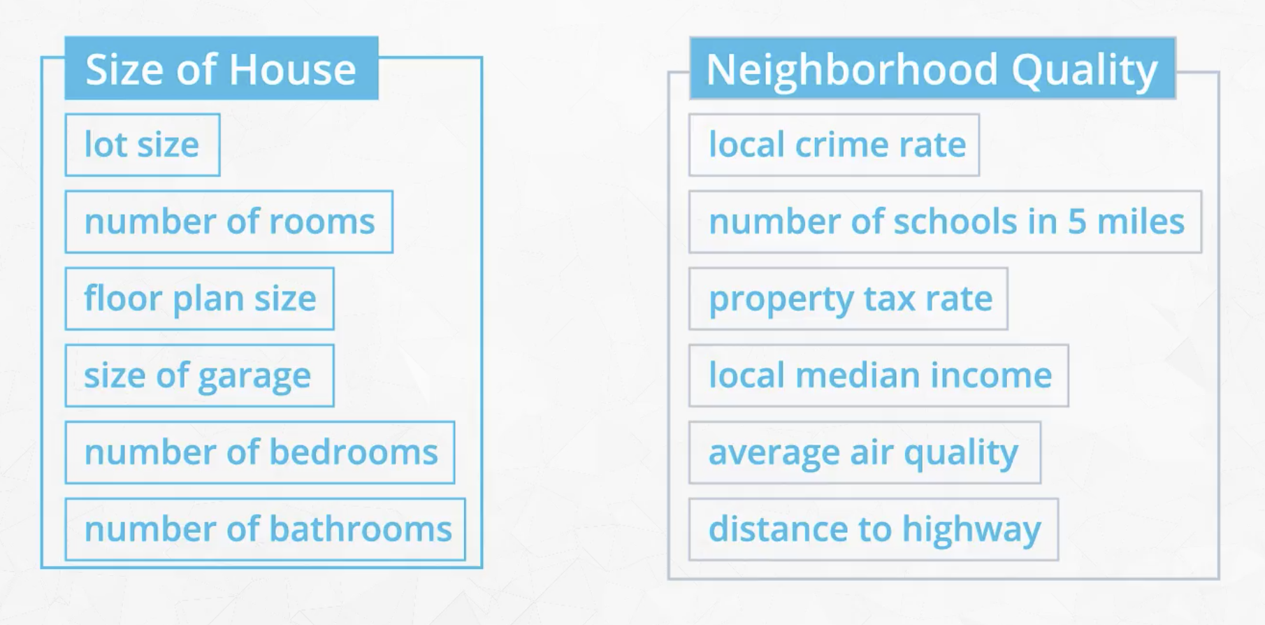
So even if our original dataset has the 12 features listed, we might be able to reduce this to only 2 latent features relating to the home size and home neighborhood.

Dimensionality Reduction through Feature Selection and Feature Extraction

Feature Selection

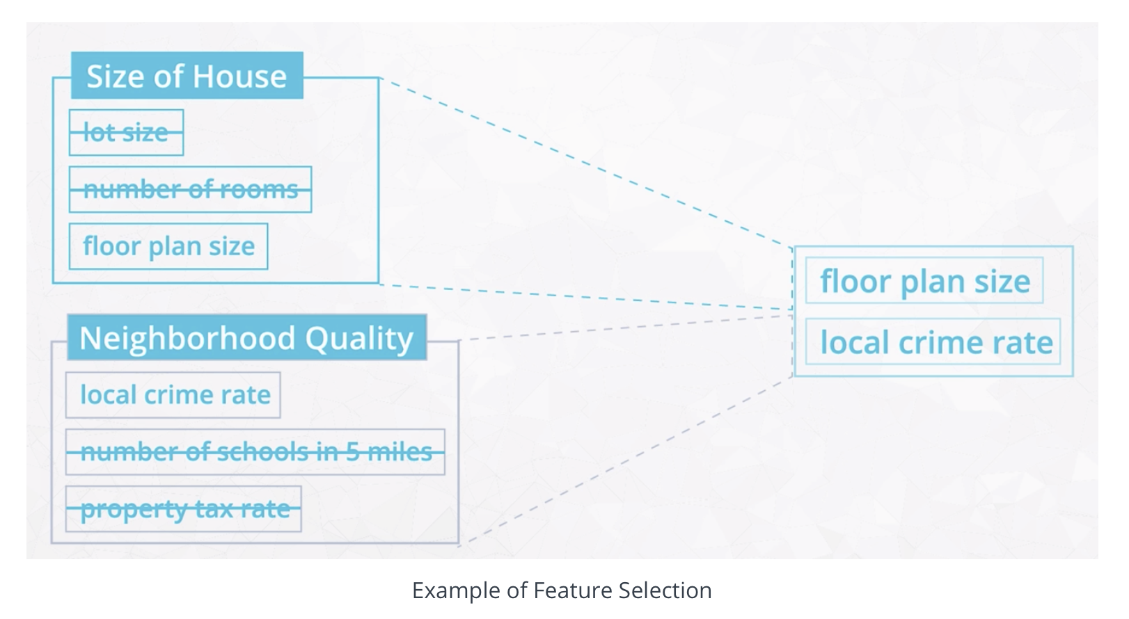
In the example above, one possible approach would be to simply select a subset of the available features as a proxy for the two identified latent features.

There are also algorithmic approaches to selecting the most appropriate fields. In general, these methods fall into two broad categories:

Filter methods - Filtering approaches use a ranking or sorting algorithm to filter out those features that have less usefulness. Filter methods are based on discerning some inherent correlations among the feature data in unsupervised learning, or on correlations with the output variable in supervised settings. Filter methods are usually applied as a preprocessing step. Common tools for determining correlations in filter methods include:

• Pearson’s Correlation,
• Linear Discriminant Analysis (LDA), and
• Analysis of Variance (ANOVA).

Wrapper methods - Wrapper approaches generally select features by directly testing their impact on the performance of a model. The idea is to “wrap” this procedure around your algorithm, repeatedly calling the algorithm using different subsets of features, and measuring the performance of each model. Cross-validation is used across these multiple tests. The features that produce the best models are selected. Clearly this is a computationally expensive approach for finding the best performing subset of features, since they have to make a number of calls to the learning algorithm. Common examples of wrapper methods are:

• Forward Search,
• Backward Search, and
• Recursive Feature Elimination.

Scikit-learn has a feature selection module that offers a variety of methods to improve model accuracy scores or to boost their performance on very high-dimensional datasets.

Feature Extraction

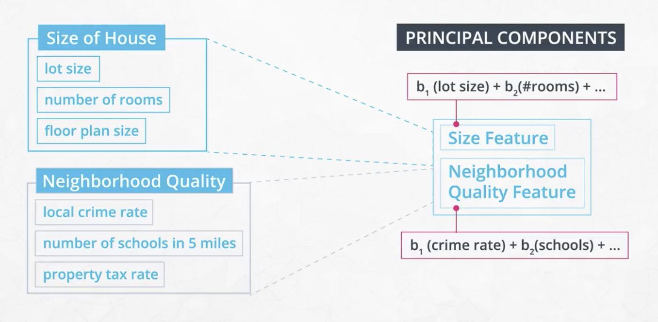
Feature Extraction involves extracting, or constructing, new features called latent features. In the example image below, taken from the video, “Size Feature” and “Neighborhood Quality Feature” are new latent features, extracted from the original input data.

Methods for feature extraction include:

• Principal Component Analysis (PCA),
• Independent Component Analysis (ICA), and
• Random Projection.

Other Resources

• Introduction to Feature Selection methods
• Dimensionality Reduction Algorithms: Strengths and Weaknesses
• An Introduction to Variable and Feature Selection
• Info on Best Practices for selecting an appropriate number of components

Feature Extraction using PCA

Feature Extraction is generally preferred to Feature Selection because the latent features can be constructed to incorporate data from multiple features, and thus retain more information present in the various original inputs, than just losing that information by dropping many original inputs.

Principal Components are linear combinations of the original features in a dataset that aim to retain the most information in the original data. Principal components are conceptually similar to latent features in that they combine multiple features into a single aggregate feature.

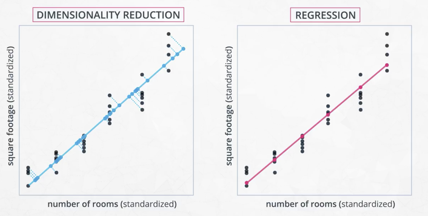
To help understand this, consider for example the relationship between square footage and number of rooms.

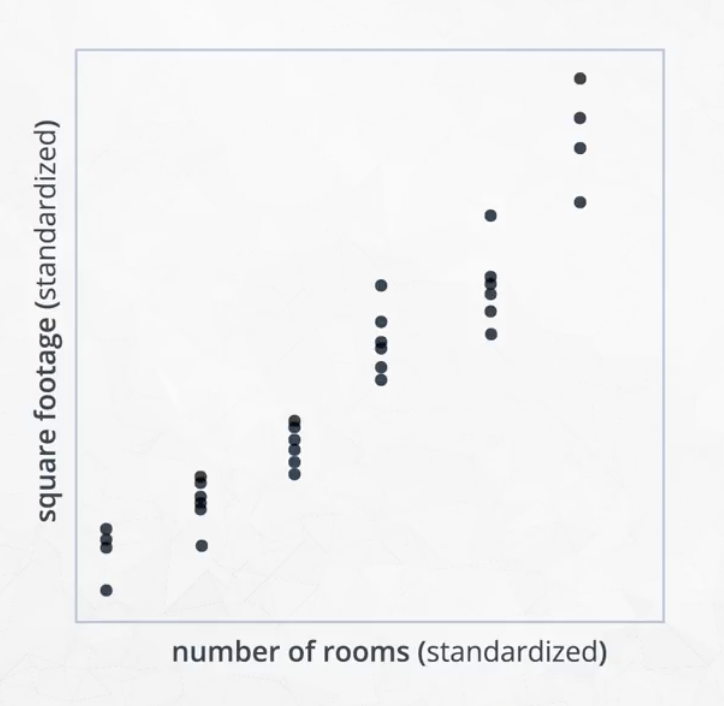
This two-dimensional data can be reduced to a single dimension through the line shown in the image on the left, below. Conceptually, this is very similar to regression, except that the goal is not to make a prediction, but to shrink the space that the data lives in.

The general approach to this problem of high-dimensional datasets is to search for a projection of the data onto a smaller number of features which preserves the information as much as possible.

There are two main properties of principal components:

1. They retain the most amount of information in the dataset. In this video, you saw that retaining the most information in the dataset meant finding a line that reduced the distances of the points to the component across all the points.
2. The created components are orthogonal to one another. So far we have been mostly focused on what the first component of a dataset would look like. However, when there are many components, the additional components will all be orthogonal to one another. Depending on how the components are used, there are benefits to having orthogonal components. In regression, we often would like independent features, so using the components in regression now guarantees this.

The amount of information lost when performing PCA is the distance from the original points to the created component.

PCA Mathematics

The mathematics of PCA isn’t really necessary for PCA to be useful. However, it can be useful to fully understand the mathematics of a technique to understand how it might be extended to new cases.

A simple introduction of what PCA is aimed to accomplish is provided here in a simple example on YouTube.

A nice visual, and mathematical, illustration of PCA is provided in this video by 3 blue 1 brown.

An eigenvalue is the same as the amount of variability captured by a principal component, and an eigenvector is the principal component itself. To see more on these ideas, take a look at the following three links below:

• PDF Tutorial
• Great Tutorial using Iris Dataset
• SKLearn Documentation Example using Faces

Where is PCA Used?

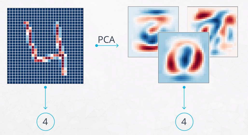
In general, PCA is used to reduce the dimensionality of your data. My notes include an example where PCA is used to process image data from many pixels to just 15 features, while still maintaining almost the same accuracy as when all the pixels were kept.

Other examples might include discovering latent features in survey data to find patterns and behavioral habits.

Here are some other specific examples:

• PCA for microarray data,
• PCA for anomaly detection,
• PCA for time series data.

Fundamentally, PCA is a technique to transform data down such that in a way that helps maximize the information from the original data.

Summary

Two Methods for Dimensionality Reduction

• Feature Selection and Feature Extraction are two general approaches for reducing the number of features in your data. Feature Selection processes result in a subset of the most significant original features in the data, while Feature Extraction methods like PCA construct new latent features that well represent the original data.

Dimensionality Reduction and Principal Components

• Principal Component Analysis (PCA) is a technique that is used to reduce the dimensionality of your dataset. The reduced features are called principal components, or latent features. These principal components are simply a linear combination of the original features in your dataset.

That these components have two major properties:

1. They aim to capture the most amount of variability in the original dataset.
2. They are orthogonal to (independent of) one another.

Fitting PCA

Other notes I have on this subject show a function called do_pca, which returned the PCA model, as well as the reduced feature matrix. It takes as parameters number of features needed back, as well as the original dataset.

Interpreting Results

There are two major parts to interpreting the PCA results:

1. The variance explained by each component. You were able to visualize this with scree plots to understand how many components you might keep based on how much information was being retained.
2. The principal components themselves, which gave us an idea of which original features were most related to why a component was able to explain certain aspects about the original datasets.

Here’s a well-written summary of PCA for a layman audience.