Naive Bayes
Naive Bayes is a more probabilistic algorithm that is based on the concept of conditional probability. Compared to other ML algorithms, it is easy to implement and fast to train.
Real-World Example
Consider the following example. Suppose you are in an office and happen to see someone pass by very quickly. You know that it was either Alex or Brenda, but you were unable to see which. You know that Alex and Brenda are in the office at the same amount of time per week. Given just this information, the probability that it was Alex is the same as the probability that it was Brenda.
$$P_{Alex} = P_{Brenda} = 0.5$$
Suppose that you happen to notice that the person who rushed by was wearing a red sweater. Having known both Alex and Brenda for a long time, you happen to know that Alex wears a red sweater 2 day per week, whereas Brenda wears a red sweater 3 days per week.
$$P_{Alex} = 0.40;\ P_{Brenda} = 0.60$$
This is Bayes' Theorem in a nutshell. The “prior” guess is $P_{Alex} = P_{Brenda} = 0.5$. With the additional information about the sweater, we make the “posterior” guess of $P_{Alex} = 0.4;\ P_{Brenda} = 0.6$. It is called the posterior because we make the guess after the new information has arrived.
Known versus Inferred
Fundamentally, Bayes' Theorem empowers us to switch from what we know to what we infer.
In the case of the previous example, know the probability that Alex wears red and the probability that Brenda wears red. We infer the probability that the person wearing red is Alex and the probability that the person wearing red is Brenda.
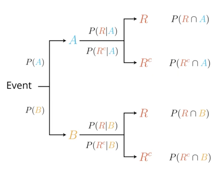
More technically, we initially know the probability of an event $A$: $P(A)$. To give us more information, we introduce an event $R$ related to event $A$. Then, we know the probability of $R$ given $A$: $P(R|A)$.
Bayes' Theorem allows us to infer the probability of $A$ given $R$: $P(A|R)$.
Revisiting the Real-World Example
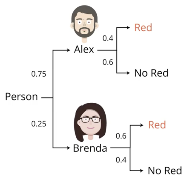
Now assume that Alex and Brenda are not in the office the same amount of time per week. Specifically, assume that Alex is in the office 3 days per week while Brenda is only in the office 1 day per week. They still wear their red sweaters with the same probabilities as before, however.
$$P_{Alex} = 0.75;\ P_{Brenda} = 0.25$$
Recall that $P(A\ and\ B) = P(A) \times P(B)$. Then, the probability that we would see Alex and that he would be wearing red is $P_{Alex,Red}=(0.75)(0.4)=0.3$.
| # | Probability | Calculation |
|---|---|---|
| 1 | $P_{Red|Alex}$ | (0.75)(0.4) = 30% |
| 2 | $P_{not\ Red|Alex}$ | (0.75)(0.6) = 45% |
| 3 | $P_{Red|Brenda}$ | (0.25)(0.6) = 15% |
| 4 | $P_{not\ Red|Brenda}$ | (0.25)(0.4) = 10% |
Note that the probabilities in the table above add up to 100%. But, we know that the person was wearing red, and this is where the magic of Bayes' Theorem comes in. We can discard situations 2 and 4 in the table above, entirely. So, we rebase the probabilities in terms of just those two situations.
$$P(Alex|Red)=\frac{0.75 \times 0.4}{0.75 \times 0.4 + 0.25 \times 0.6}=67%$$
$$P(Brenda|Red)=\frac{0.25 \times 0.4}{0.75 \times 0.4 + 0.25 \times 0.6}=33%$$
Formalized Bayes' Theorem
The Law of Conditional Probability dictates
$$P(R \cap A) = P(A) P(R|A)$$
From this we can derive Bayes' Theorem, which is
$$P(A|R) = \frac{P(A)P(R|A)}{P(A)P(R|A) + P(B)P(R|B)}$$
The more common formulation is
$$P(B|A) = \frac{P(A|B)P(B)}{P(A)}$$
Bayes' Theorem and False Positives
Consider the following application of Bayes' Theorem. Suppose that you are feeling sick and head to the doctor. The doctor suspects you of a particular disease and administers a test with the following characteristics:
- 99% “accuracy”
- Correctly diagnoses 99 out of 100 sick patients (“sensitivity”)
- Correctly diagnoses 99 out of 100 healthy patients (“specificity”)
The doctor also informs you that 1 out of every 10,000 people suffer from the disease.
Notationally, this can be written as:
- $P(S) = 0.0001$
- $P(H) = 0.9999$
- $P(+|S) = 0.99$
- $P(+|H) = 0.01$
Now, apply Bayes' Theorem:
$$P(S|+) = \frac{P(S)P(+|S)}{P(S)P(+|S) + P(H)P(+|H)}$$
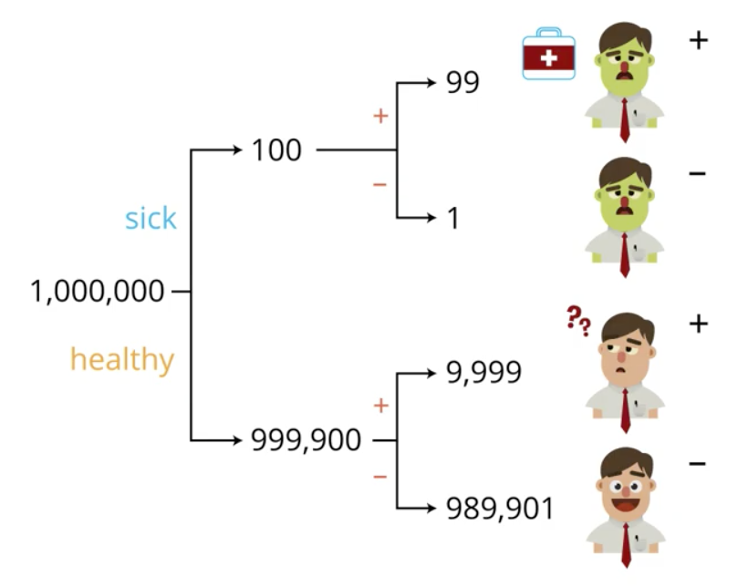
$$P(S|+) = \frac{0.0001 \times 0.99}{0.0001 \times 0.99 + 0.999 \times 0.01} = 0.0098 < 1%$$
The reason for this is made more intuitive in the following image. Since you tested positive, you are among the 10,098 people in the image with a positive test result. A very large majority of these are healthy people who tested false positive.
Example from Spam Emails
Assume that we have spam emails with the following subjects:
- Win money now!
- Make cash easy!
- Cheap money, reply!
Assume that we also have normal emails with the following subjects:
- How are you?
- There you are
- Can I borrow money?
- Say hi to grandma.
- Was the exam easy?
Using what is known, we can answer:
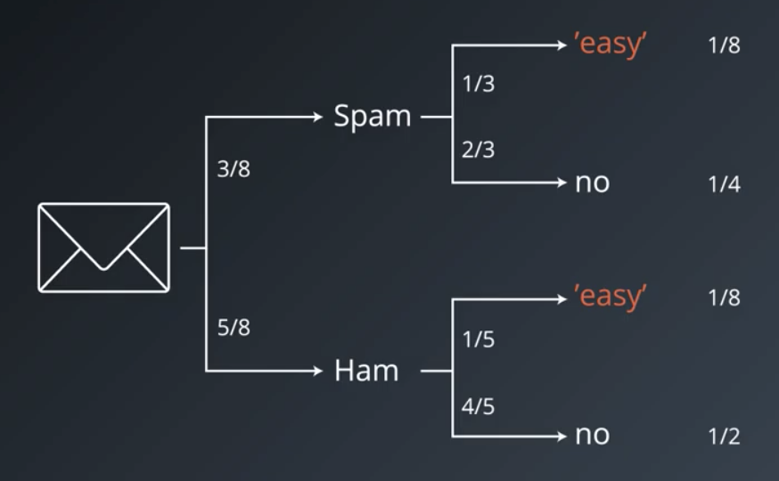
- What is the probability that an e-mail contains the word “easy”, given that it is spam? $$P(“easy”|spam)=\frac{1}{3}$$
- What is the probability that an e-mail contains the word “money”, given that it is spam? $$P(“money”|spam)=\frac{2}{3}$$
Using what we can infer, we can answer:
- What is the probability that an email is spam, given that it contains the word “easy”? $$P(spam|“easy”)=\frac{1}{2}$$
- What is the probability that an email is spam, given that it contains the word “money”? $$P(spam|“money”)=\frac{2}{3}$$
The “Naive” in Naive Bayes
Naive Bayes makes the naive assumption that the two events under consideration are independent of one another. The $\cap$ symbol below stands for “intersection.”
As an example, consider that the probability of it being hot outside is some small probability ($P(hot)>0$). Likewise, there is some small probability that it is cold outside ($P(cold)>0$). But, it does not follow that $P(hot \cap cold)>0$, because $P(hot \cap cold) \neq P(hot)P(cold)$. It isn’t possible for it to be both hot and cold simultaneously, so the events are not independent.
So, $P(A)$ and $P(B)$, below, are only be multiplied together in the event that the events are independent.
$$Independent\ only:\ P(A \& B)=P(A \cap B)=P(A)P(B)$$
Rearrange Baye’s Theorem from above
$$P(A|B)P(B) = P(B|A)P(A)$$
If we disregard $P(B)$, then we can still say the following
$$P(A|B) \propto P(B|A)P(A)$$
Apply the formula above to the spam email example.
$$P(spam|“easy”,“money”) \propto P(“easy”,“money”|spam) P(spam)$$
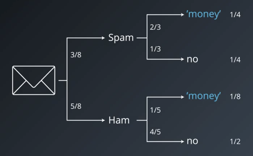
Using the naive assumption from above, and then plugging in the ratios we had from before:
$$P(“easy”,“money”|spam)=P(“easy”|spam)P(“money”|spam)$$ $$P(spam|“easy”,“money”) \propto P(“easy”|spam) P(“money”|spam) P(spam)$$ $$P(spam|“easy”,“money”) \propto \frac{1}{3} \times \frac{2}{3} \times \frac{3}{8} = \frac{1}{12}$$
Likewise, for legitimate (“ham”) emails:
$$P(ham|“easy”,“money”) \propto P(“easy”|ham) P(“money”|ham) P(ham)$$ $$P(ham|“easy”,“money”) \propto \frac{1}{5} \times \frac{1}{5} \times \frac{5}{8} = \frac{1}{40}$$
Since we know that the email must be either spam or a legitimate email, we can normalize these fractions to be $\frac{10}{13}$ and $\frac{3}{13}$, respectively. This normalization step is accomplished by dividing each of the fractions by the sum of both.
$$\frac{\frac{1}{12}}{\frac{1}{12}+\frac{1}{40}}=\frac{\frac{1}{12}}{\frac{40+12}{480}} =\frac{1}{12} \times \frac{480}{52}=\frac{40}{52}=\frac{10}{13}$$
Dice Example
Someone has a bag with
- 3 standard dice (face values: 1, 2, 3, 4, 5, 6) and
- 2 trick dice (face values: 2, 3, 3, 4, 4, 5).
Suppose they draw a die from the bag, roll it, and get a 3. What is the probability that the die was a standard die?
$$P(A|B) \propto P(B|A)P(A)$$
$$P(standard|\ 3\ ) \propto P(\ 3\ |standard) P(standard) = \frac{1}{6} \times \frac{3}{5}=\frac{1}{10}$$ $$P(trick|\ 3\ ) \propto P(\ 3\ |trick) P(trick) = \frac{1}{3} \times \frac{2}{5} = \frac{2}{15}$$ $$P(standard|\ 3\ )=\frac{\frac{1}{10}}{\frac{1}{10}+\frac{2}{15}}=\frac{\frac{1}{10}}{\frac{15+20}{150}} = \frac{1}{10} \times \frac{150}{35}=\frac{3}{7}$$