Linear Regression Implementations
Implementing Mini-Batch Gradient Descent Using Numpy
%matplotlib inline
%config InlineBackend.figure_format = 'retina'

import numpy as np
np.random.seed(42)
import matplotlib.pyplot as plt
$$\hat{y} = Wx + b$$
$$Error = \frac{1}{2m} \sum^m_{i=1}(y-\hat{y})^2$$
$$\frac{\partial}{\partial W} Error = \frac{\partial Error}{\partial \hat{y}} \frac{\partial \hat{y}}{\partial W} = -(y-\hat{y})x$$
$$\frac{\partial}{\partial b} Error = \frac{\partial Error}{\partial \hat{y}} \frac{\partial \hat{y}}{\partial b} = -(y-\hat{y})$$
$$W \rightarrow W - \alpha \frac{\partial}{\partial W} Error$$
def MSEStep(X, y, W, b, learn_rate = 0.005):
    """
    This function implements the gradient descent step for squared error as a
    performance metric.

    Parameters
    X : array of predictor features
    y : array of outcome values
    W : predictor feature coefficients
    b : regression function intercept
    learn_rate : learning rate

    Returns
    W_new : predictor feature coefficients following gradient descent step
    b_new : intercept following gradient descent step
    """
    y_pred = np.matmul(X, W) + b
    error = y - y_pred

    W_new = W + learn_rate * np.matmul(error, X)
    b_new = b + learn_rate * error.sum()

    return W_new, b_new
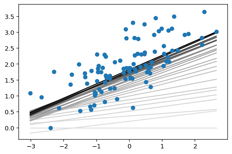
# The gradient descent step will be performed multiple times on
# the dataset, and the returned list of regression coefficients
# will be plotted.
def miniBatchGD(X, y, batch_size = 20, learn_rate = 0.005, num_iter = 25):
    """
    This function performs mini-batch gradient descent on a given dataset.

    Parameters
    X : array of predictor features
    y : array of outcome values
    batch_size : how many data points will be sampled for each iteration
    learn_rate : learning rate
    num_iter : number of batches used

    Returns
    regression_coef : array of slopes and intercepts generated by gradient
      descent procedure
    """
    n_points = X.shape[0]
    W = np.zeros(X.shape[1]) # coefficients
    b = 0 # intercept

    # run iterations
    regression_coef = [np.hstack((W,b))]
    for _ in range(num_iter):
        batch = np.random.choice(range(n_points), batch_size)
        X_batch = X[batch,:]
        y_batch = y[batch]
        W, b = MSEStep(X_batch, y_batch, W, b, learn_rate)
        regression_coef.append(np.hstack((W,b)))

    return regression_coef
# perform gradient descent
data = np.loadtxt('linear-regression-implementations/data.csv',
                  delimiter = ',')
X = data[:,:-1]
y = data[:,-1]

regression_coef = miniBatchGD(X, y)

plt.figure()
X_min = X.min()
X_max = X.max()
counter = len(regression_coef)
for W, b in regression_coef:
    counter -= 1
    color = [1 - 0.92 ** counter for _ in range(3)]
    plt.plot([X_min, X_max],[X_min * W + b, X_max * W + b], color = color)
plt.scatter(X, y, zorder = 3)
plt.show()
Linear Regression on a Dataset from Gapminder
import pandas as pd
from sklearn.linear_model import LinearRegression
filepath = 'linear-regression-implementations/bmi_and_life_expectancy.csv'
bmi_life_data = pd.read_csv(filepath)
bmi_life_data.head()
| Country | Life expectancy | BMI | |
|---|---|---|---|
| 0 | Afghanistan | 52.8 | 20.62058 |
| 1 | Albania | 76.8 | 26.44657 |
| 2 | Algeria | 75.5 | 24.59620 |
| 3 | Andorra | 84.6 | 27.63048 |
| 4 | Angola | 56.7 | 22.25083 |
x_values = (bmi_life_data['BMI']
            .values
            .reshape(-1, 1))
y_values = (bmi_life_data['Life expectancy']
            .values
            .reshape(-1, 1))

bmi_life_model = LinearRegression()
bmi_life_model.fit(x_values, y_values)

laos_life_exp = bmi_life_model.predict([[21.07931]])
laos_life_exp
array([[60.31564716]])
Linear Regression on the Boston Housing Dataset
The Boston dataset consists of 13 features of 506 houses as well as the median home value in thousands of dollars.
from sklearn.datasets import load_boston
from sklearn.linear_model import LinearRegression
boston_data = load_boston()
x = boston_data['data']
y = boston_data['target']

print(x.shape, y.shape)
(506, 13) (506,)
boston_model = LinearRegression().fit(x, y)

sample_house = [[2.29690000e-01, 0.00000000e+00, 1.05900000e+01,
                 0.00000000e+00, 4.89000000e-01, 6.32600000e+00,
                 5.25000000e+01, 4.35490000e+00, 4.00000000e+00,
                 2.77000000e+02, 1.86000000e+01, 3.94870000e+02,
                 1.09700000e+01]]
prediction = boston_model.predict(sample_house)
prediction
array([23.68284712])
Polynomial Regression
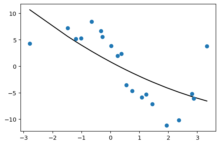
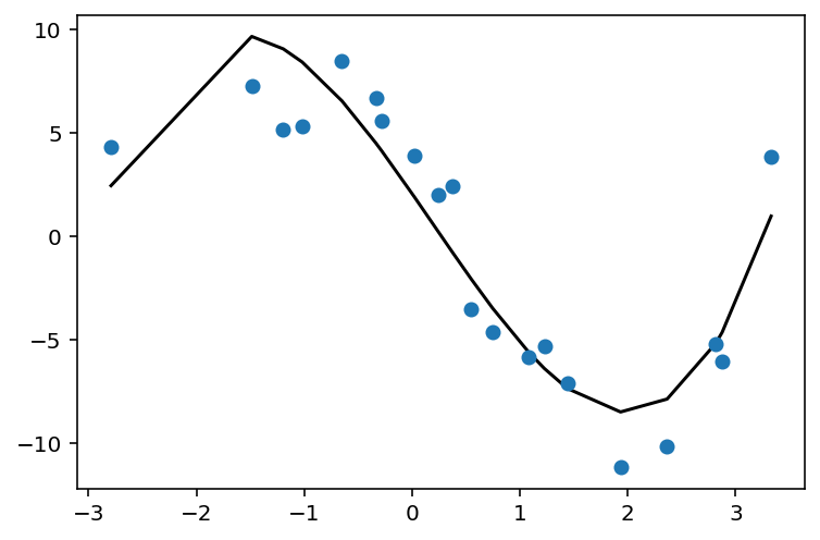
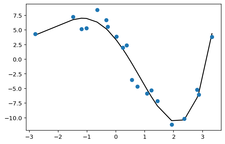
The dataset is small (20 samples) and nonlinear.
import pandas as pd
from sklearn.linear_model import LinearRegression
from sklearn.preprocessing import PolynomialFeatures
filepath = 'linear-regression-implementations/poly-reg-data.csv'
poly_reg_data = (pd.read_csv(filepath)
                 .sort_values(['Var_X'])
                 .reset_index(drop=True))

print(poly_reg_data.shape)
poly_reg_data.head()
(20, 2)
| Var_X | Var_Y | |
|---|---|---|
| 0 | -2.79140 | 4.29794 |
| 1 | -1.48662 | 7.22328 |
| 2 | -1.19438 | 5.16161 |
| 3 | -1.01925 | 5.31123 |
| 4 | -0.65046 | 8.43823 |
X = (poly_reg_data['Var_X']
     .values
     .reshape(-1, 1))
y = (poly_reg_data['Var_Y']
     .values
     .reshape(-1, 1))
print(X.shape, y.shape)
(20, 1) (20, 1)
Degree 2: $w_1 X^2 + w_2 X + w_3$
Degree 3: $w_1 X^3 + w_2 X^2 + w_3 X + w_4$
Degree 4: $w_1 X^4 + w_2 X^3 + w_3 X^2 + w_4 X + w_5$
def fit_and_plot_poly_deg(degree):
    poly_feat = PolynomialFeatures(degree)
    X_poly = poly_feat.fit_transform(X)

    print('X_poly shape is: {}'.format(str(X_poly.shape)))

    poly_model = LinearRegression().fit(X_poly, y)
    y_pred = poly_model.predict(X_poly)

    plt.scatter(X, y, zorder=3)
    plt.plot(X, y_pred, color='black');
fit_and_plot_poly_deg(2)
X_poly shape is: (20, 3)
fit_and_plot_poly_deg(3)
X_poly shape is: (20, 4)
fit_and_plot_poly_deg(4)
X_poly shape is: (20, 5)
Regularization with Lasso
import pandas as pd
from sklearn.linear_model import Lasso
filepath = 'linear-regression-implementations/lasso_data.csv'
lasso_data = pd.read_csv(filepath,
                         header=None)
print(lasso_data.shape)
lasso_data.head()
(100, 7)
| 0 | 1 | 2 | 3 | 4 | 5 | 6 | |
|---|---|---|---|---|---|---|---|
| 0 | 1.25664 | 2.04978 | -6.23640 | 4.71926 | -4.26931 | 0.20590 | 12.31798 |
| 1 | -3.89012 | -0.37511 | 6.14979 | 4.94585 | -3.57844 | 0.00640 | 23.67628 |
| 2 | 5.09784 | 0.98120 | -0.29939 | 5.85805 | 0.28297 | -0.20626 | -1.53459 |
| 3 | 0.39034 | -3.06861 | -5.63488 | 6.43941 | 0.39256 | -0.07084 | -24.68670 |
| 4 | 5.84727 | -0.15922 | 11.41246 | 7.52165 | 1.69886 | 0.29022 | 17.54122 |
X = (lasso_data[lasso_data.columns[0:6]]
     .values)
y = (lasso_data[lasso_data.columns[6]]
     .values)
print(X.shape, y.shape)
(100, 6) (100,)
lasso_reg = Lasso().fit(X, y)
lasso_reg.coef_
array([ 0.        ,  2.35793224,  2.00441646, -0.05511954, -3.92808318,
        0.        ])
Lasso used regularization to zero out the coefficients for two of the input features, columns 0 and 6.
Standardization
This example uses the same data as in the “Regularization with Lasso” example above, except it standardizes it.
from sklearn.preprocessing import StandardScaler
X = (lasso_data[lasso_data.columns[0:6]]
     .values)
y = (lasso_data[lasso_data.columns[6]]
     .values)
print(X.shape, y.shape)
(100, 6) (100,)
scaler = StandardScaler()

X_scaled = scaler.fit_transform(X)
lasso_reg = Lasso().fit(X_scaled, y)
lasso_reg.coef_
array([  0.        ,   3.90753617,   9.02575748,  -0.        ,
       -11.78303187,   0.45340137])
Note that following regularization, Lasso has zeroed out the coefficients for different columns, namely 0 and 4 rather than 0 and 6.
This is an example of why it is important to apply feature scaling before using regularization techniques.