Ensemble Methods
Ensemble methods are ways of joining several methods together in order to get a better model. Two of the most popular ensemble methods are:
- Bagging, short for “bootstrap aggregating,” and
- Boosting.
Both will be illustrated by the analogy of several friends collaborating on a take-home, multi-subject, true/false exam.
Bagging
In the analogy, each friend will take the test separately, and then their answers will be combined to form the final answer on the exam. There are many ways of combining the answers, but the most common way is voting.
Boosting
In the analogy, boosting is similar to bagging, except it does a better job of capitalizing on each of the friends' subject area expertise. For example, if one of the friends was a math major, his answers on the math part of the test would be given greater weight than his answers on the english part, for example.
For both bagging and boosting, in this analogy, the friends are referred to as weak learners. Their combined responses are referred to as the strong learner. The weak learners are not necessarily weak. They are just referred to as such because they are joined together to form a learner that is relatively stronger.
So, bagging and boosting involve combining the outputs of several models into an output that is more accurate than any of the models individually. The individual weak learners do not need to be very good; they only need to perform better than chance.
Most commonly, the weak learners that are used in ensemble methods are decision trees. In fact, the default model in sklearn is decision trees. But, any model can be used.
Bias and Variance
The reason why it can be advantageous to combine multiple learners together is to find an appropriate balance between two competing variables in machine learning: Bias and Variance. This is commonly known as the “Bias-variance tradeoff.”
According to the wikipedia article on the subject: it is “the property of a set of predictive models whereby models with a lower bias in parameter estimation have a higher variance of the parameter estimates across samples, and vice versa.” In a nutshell, it is striking an appropriate balance between overfitting and underfitting such that the model successfully generalizes beyond the training set.
Bias
When a model has high bias, it means it doesn’t do a good job “bending to the data.” Linear regression is an algorithm that often exhibits high bias.
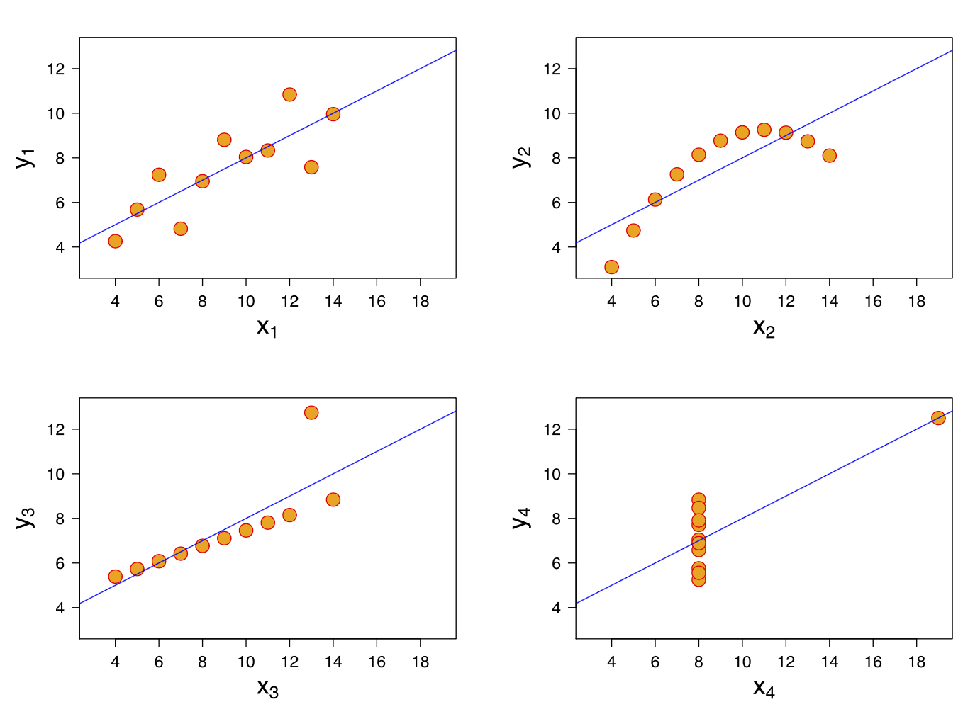
In the examples above, even with completely different datasets, we end up with the same line fit to the data.
Variance
When a model has high variance, it means it changes drastically to meet the needs of every point in the dataset. Decision trees are an algorithm that tend to have high variance, especially if they have no early stopping parameters. These “high variance” algorithms are extremely flexible to fit exactly the data they see. In the case of a decision tree, they will split every point into its own branch, if possible.
Using ensemble methods to combine algorithms, it is often possible to build models that perform better by meeting in the middle in terms of bias and variance. There are also more advanced tactics that can be used to minimize bias and variance based on mathematical theories, like the central limit theorem.
Introducing Randomness into Ensembles
There are two commonly-employed methods to introduce randomness into high variance algorithms before they are ensembled together. Introducing randomness combats the tendency of the algorithms to overfit (or even directly fit) the available data. These methods are:
- Bootstrap the data: sample the data with replacement, and fit your algorithm to the sampled data.
- Subset the features: with each decision tree split, or with each algorithm in an ensemble of algorithms, use only a subset of the total possible features.
Random forests, the algorithm introduced next, use these random components.
Random Forests
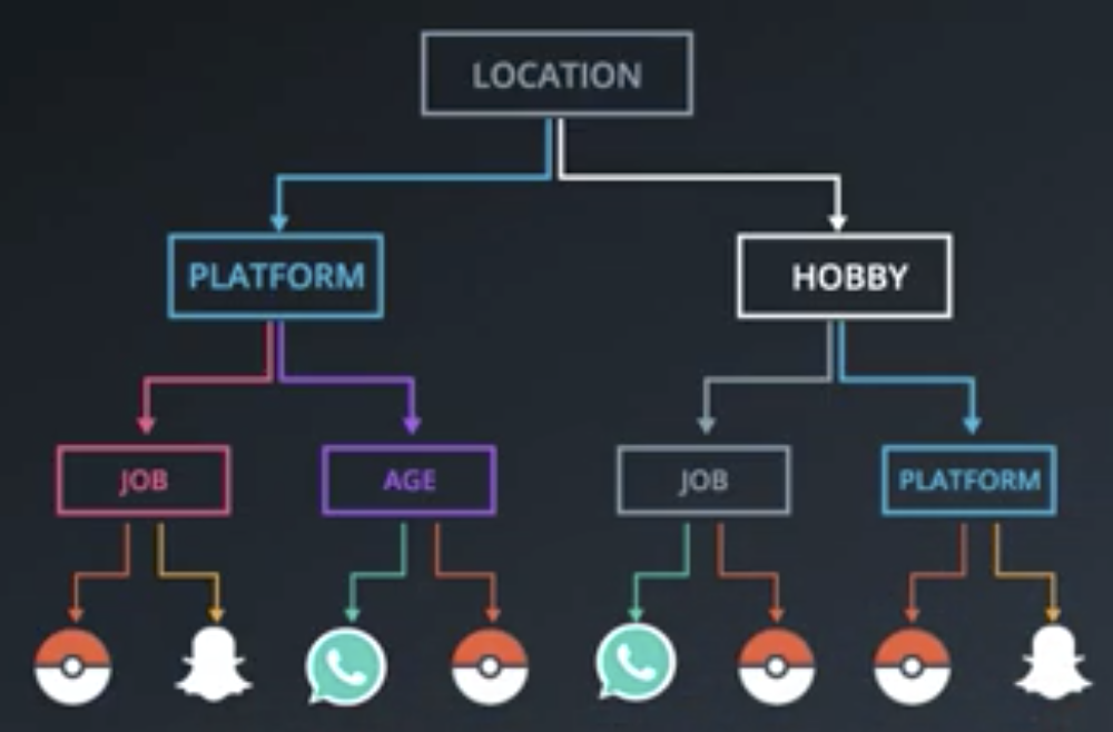
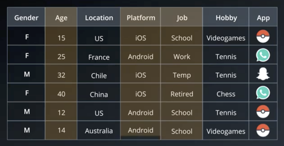
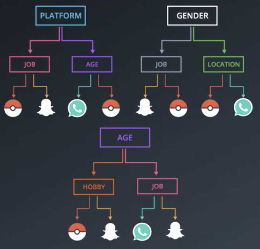
Random Forests are a means of overcoming the tendency of decision trees to overfit high-dimensional (many column) data. For example, given data like the following, a decision tree could well come up with the classification that follows the table.
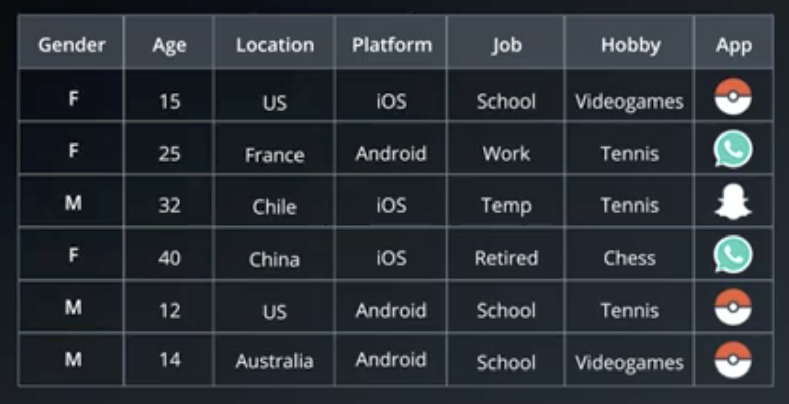
If a client is male, between 15 and 25, in the US, on Android, in school, likes tennis and pizza, but does not like long walks on the beach, then they are likely to download Pokemon Go.
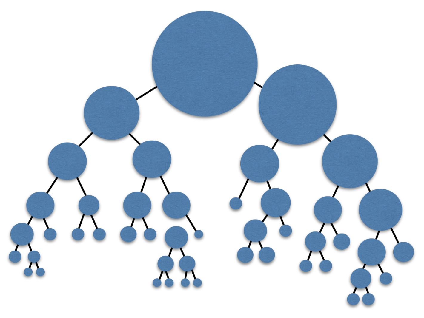
The decision tree that would come up with that classification would likely have many layers and be overfit to the data.
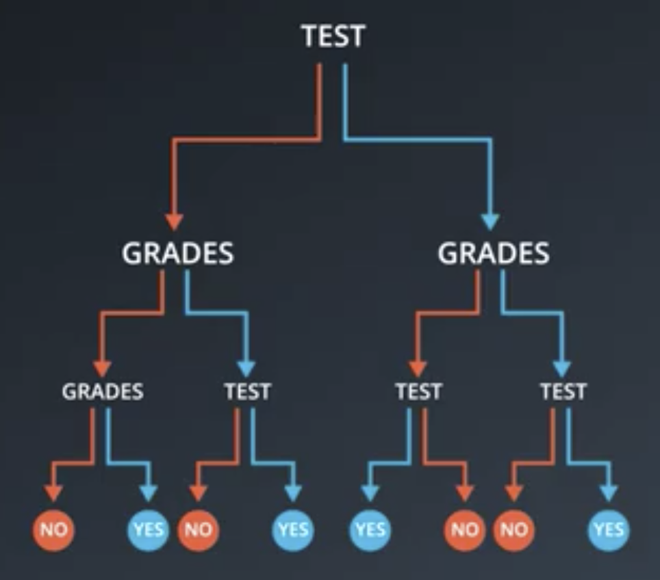
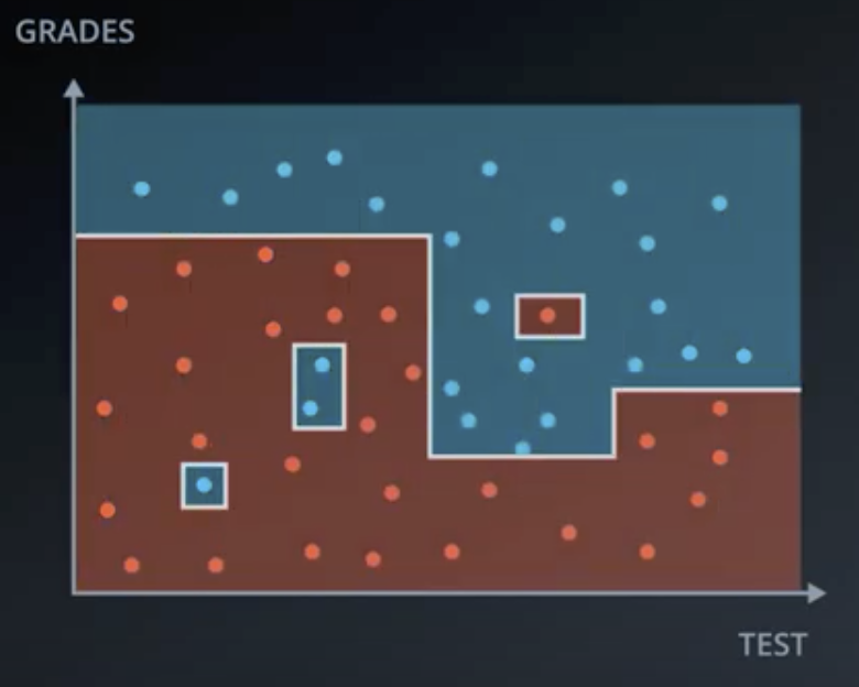
An analogous problem can arise when training a tree on continuous data.
Random Forests are a solution to these problems, whereby several smaller decisions trees are constructed, each using a subset of the available features. Then, these decision trees vote on the outcome.
There are better ways of choosing which features to train on than selecting them at random. This will be covered later.
Bagging
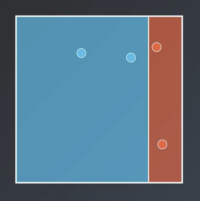
For simplicity, the weak learner in this section will be assumed to be the simplest possible learner a single-node decision tree. So, in a 2-dimensional dataset, each weak learner will be a horizontal or vertical line. Assume that the dataset resembles the following.
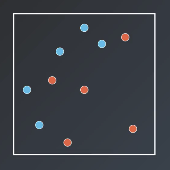
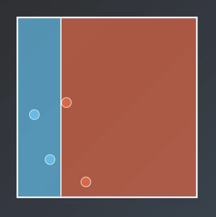
Bagging entails training each weak learner on a subset of the available data, which is computationally efficient for large datasets. So, for example the following are all possible decision trees based on the dataset shown above.
Note that, generally speaking, sampling with replacement is used and not all points need to be sampled.
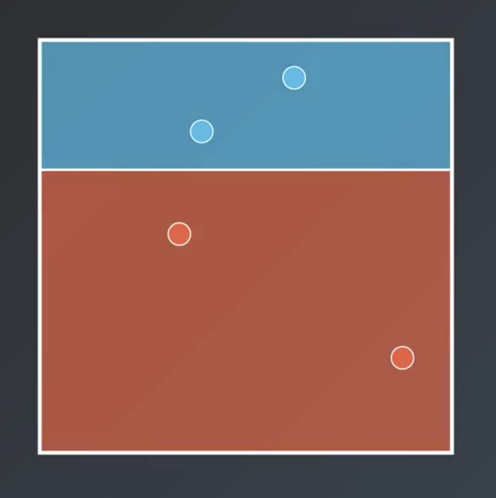
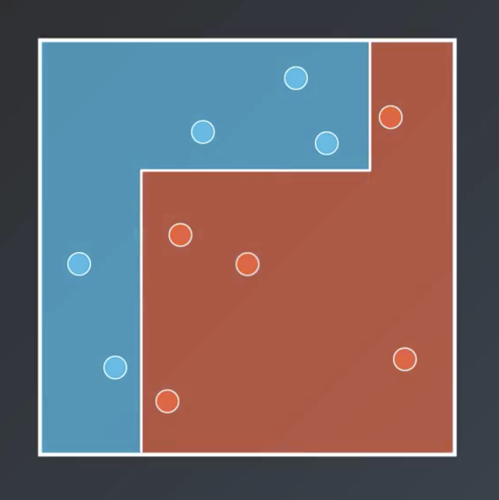
Bagging entails having each of the weak learner vote on the regions, with a result similar to that shown below.
Adaboost Overview
Adaboost, as described below, may differ slightly from the usual form described in the literature. It is, however, conceptually very similar.
Boosting, as previewed in the analogy above, is more elaborate than bagging. There are several ways to do boosting, but one of the most popular is the Adaboost algorithm which was discovered by Freund and Schapire in 1996.
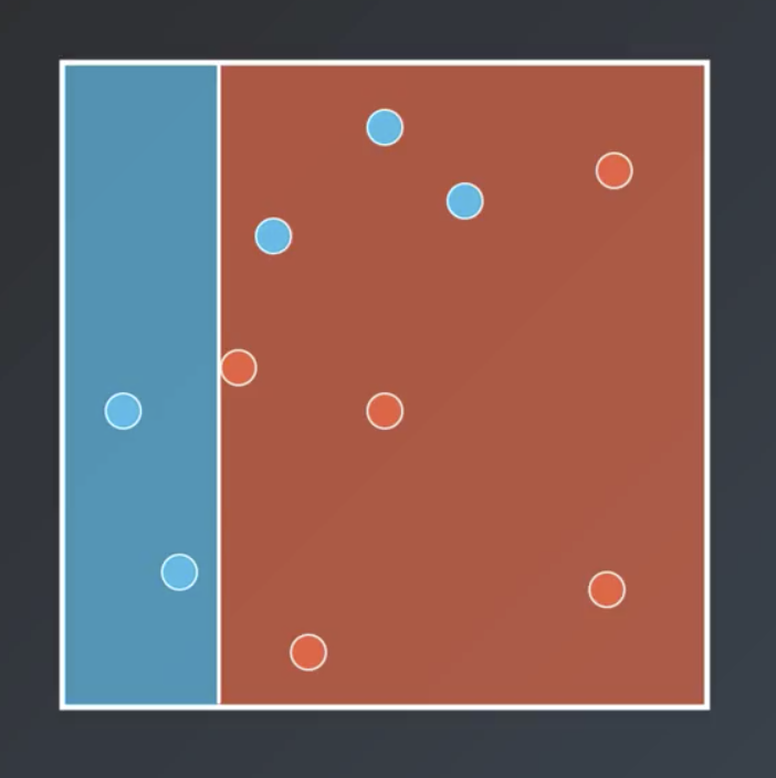
The first learner is fit in order to maximize accuracy (or, minimize errors).
The second learner should fix some of the mistakes of the first learner. To accomplish this, the weights of the points that the first classifier misclassified are increased. In other words, we add additional incentive for the next learner to correctly classify those originally-misclassified points.
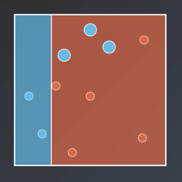
So, the next second weak learner classifies the points as follows.
The pattern repeats. The points the second classifier misclassifies are weighted more heavily. As a result, the third learner classifies the points as follows.
A more complex method for combining these three learners will be described later. For now, assume they vote on the result exactly as described previously.
Adaboost
Weighting the Data
The following is a more precise description of the algorithm that was described at a high level, above.
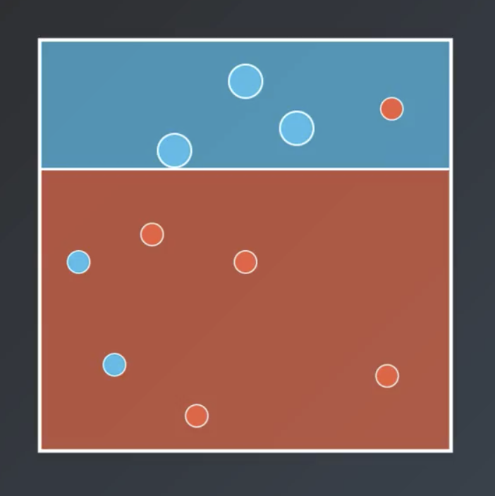
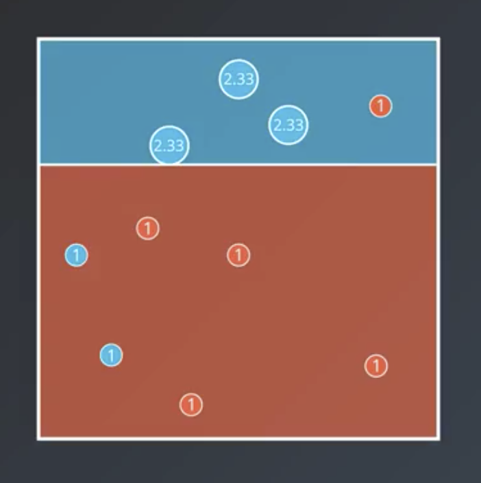
- Split the data to maximize accuracy.
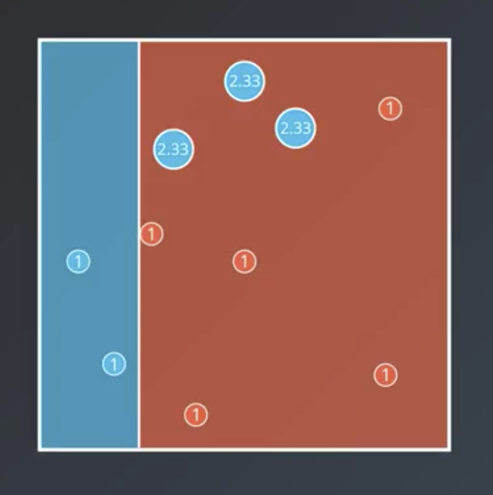
- Weight the incorrectly-classified data more heavily, such that the model becomes 50/50 correct/incorrect. In this case, it means multiplying the weights of the incorrectly-classified points by $\frac{7}{3}$ or 2.33.
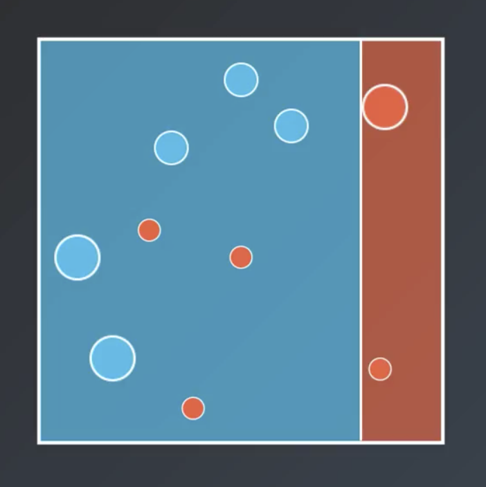
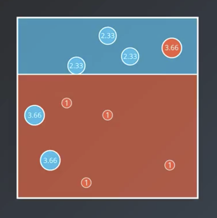
- Split the data a second time.
- Weight the incorrectly-classified data more heavily, in the same manner as before.
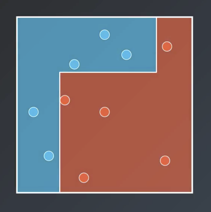
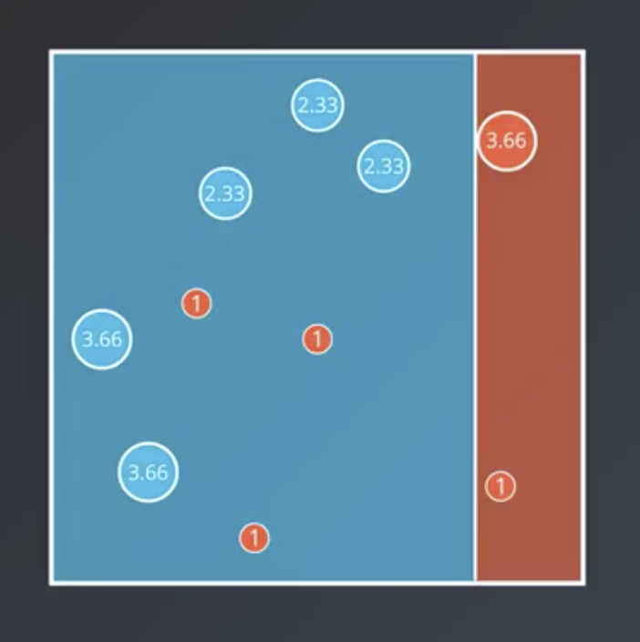
- Split the data a third time.
- The original paper by Freund and Schapire
- A follow-up paper, also by Freund and Schapire, about some experiments with Adaboost
- A tutorial by Schapire

$$Correct: 7$$ $$Incorrect: 3$$
$$Correct: 7$$ $$Incorrect: 7$$
$$Correct: 11$$ $$Incorrect: 3$$
$$Correct: 11$$ $$Incorrect: 11$$
$$Correct: 19$$ $$Incorrect: 3$$
This can be repeated further, but this is sufficient for explanatory purposes. The result so far are the following three models that will be combined in the next section.
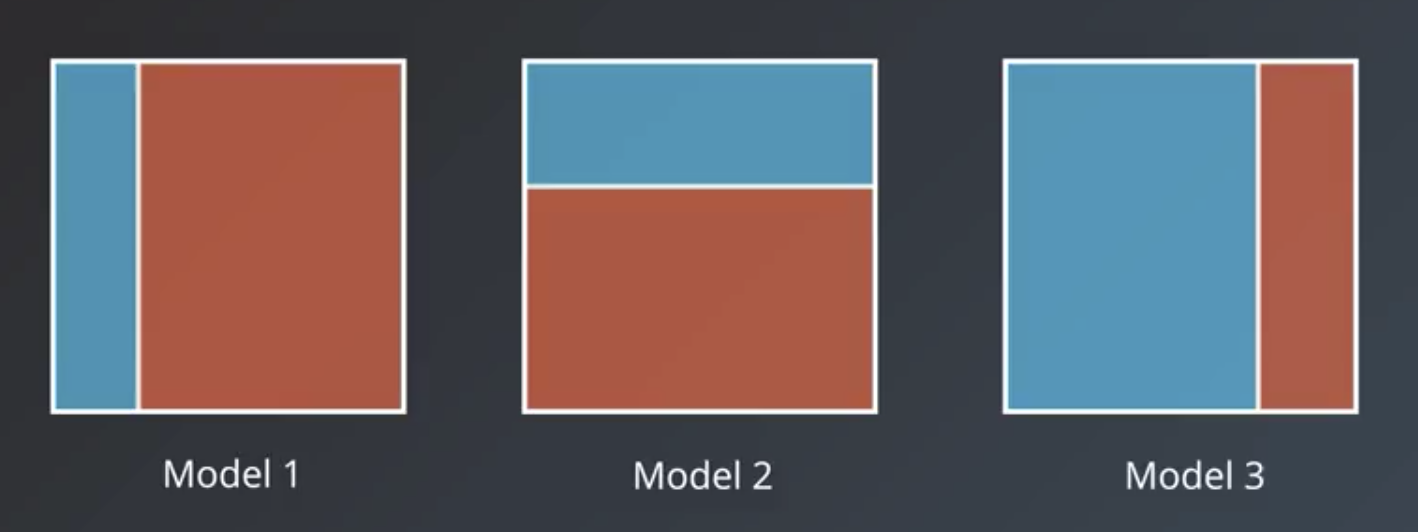
Weighting the Models
We give greater weight to the models that have the most explanatory power. Explanatory power can mean they are highly-correct (truthful) or highly-incorrect (liars). In the case of the latter group, they are given a large negative weight.
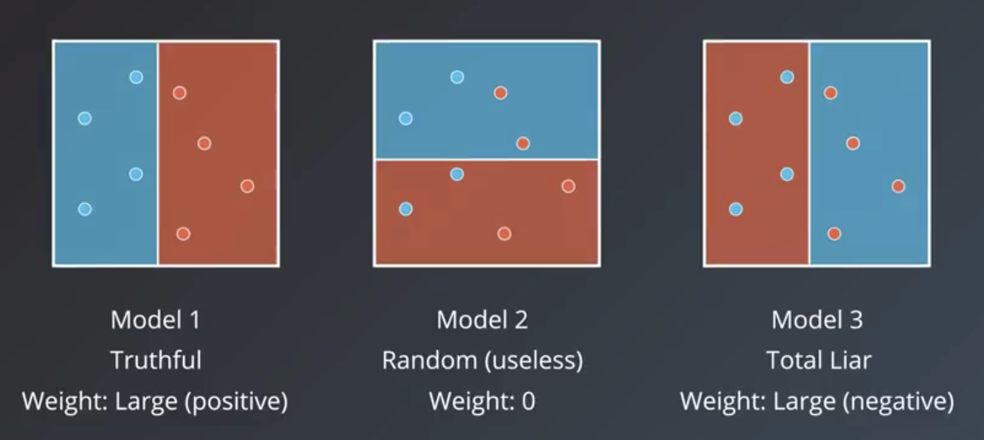
The formula that derives these weights is shown below.
$$weight = \ln(\frac{accuracy}{1-accuracy}) = \ln(\frac{\#\ correct}{\#\ incorrect})$$
The shape of the function itself follows.
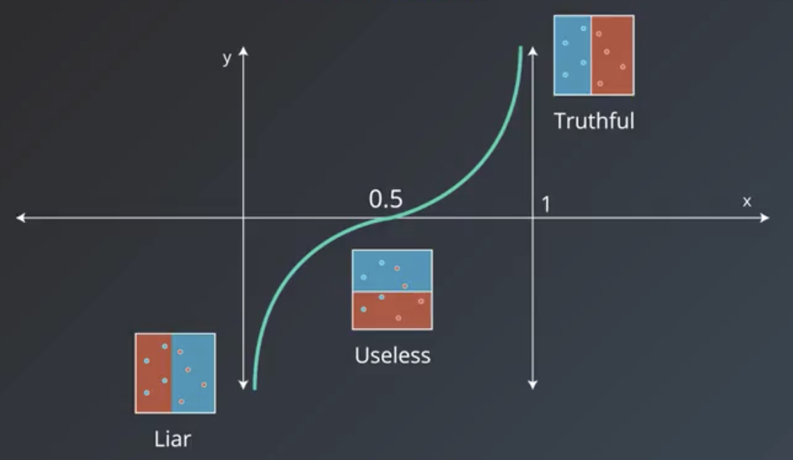
The expression for the model weight can also be written as a ratio of correct to incorrect classifications. For example, the weights of the following models are calculated below.
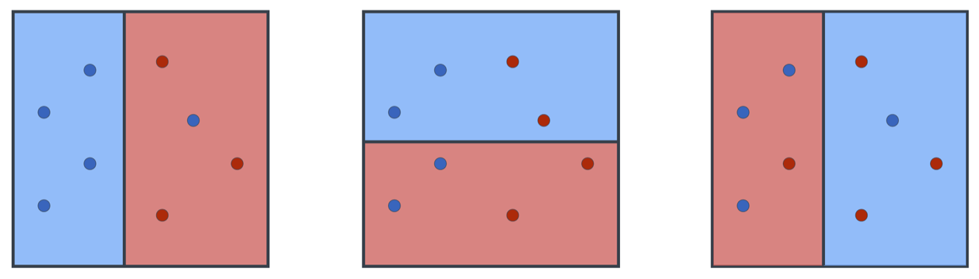
$$weight_{left} = \ln(\frac{\frac{7}{8}}{1-\frac{7}{8}}) = \ln(\frac{7}{1}) = 1.95$$
$$weight_{center} = \ln(\frac{\frac{4}{8}}{1-\frac{4}{8}}) = \ln(\frac{4}{4}) = 0$$
$$weight_{right} = \ln(\frac{\frac{2}{8}}{1-\frac{2}{8}}) = \ln(\frac{2}{6}) = -1.09$$
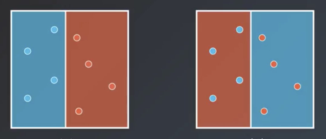
The two examples shown abbove are the bounding cases, where a weak learners classifies the data perfectly correctly or perfectly incorrectly. In this situation, the math works out to $\infty$ or $-\infty$, respectively. What this means practically is that the weights of the other learners are irrelevant and this particular weak learner should be used exclusively.
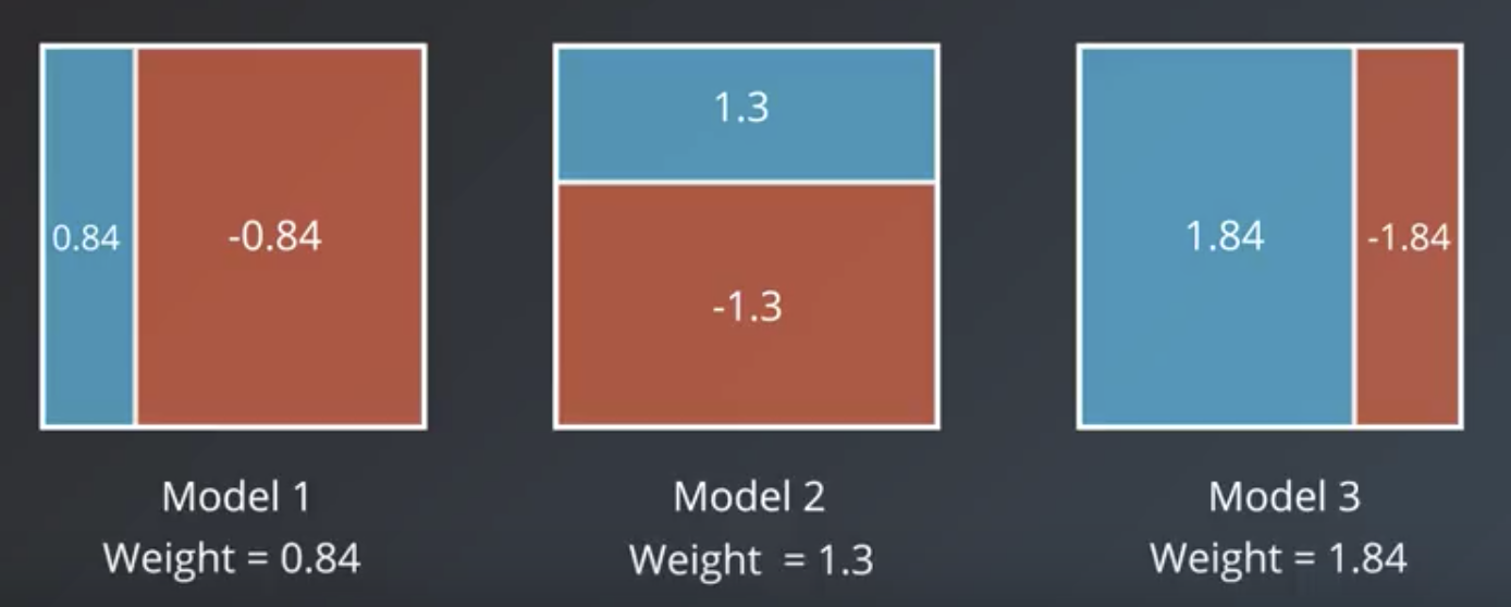
Continuing the example from above, the first weak learner, below, has $weight =\ln (\frac{7}{3}) = 0.84$.
The weight for the second one is $weight = \ln(\frac{11}{3}) = 1.3$.
The weight for the third one is $weight = \ln(\frac{19}{3}) = 1.84$.
Note that the weights do not necessarily always increase with successive iterations, as they do in this example.
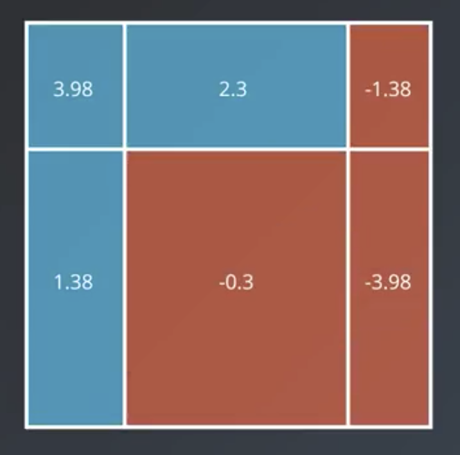
To combine the outputs of the models, we weight each model’s vote on each region by the weight of the model.
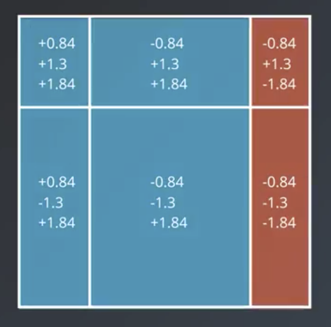
Where the result is positive, the color is blue. Where it is negative, it is red. Note that the resulting strong learner classifies the data perfectly.