Decision Trees

Decisions trees operate by asking a series of successive questions about the data until it narrows the information down well enough to make a suggestion.

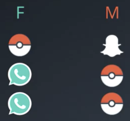
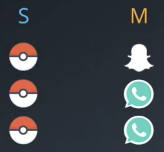
App Preferences from Demographic Data Example

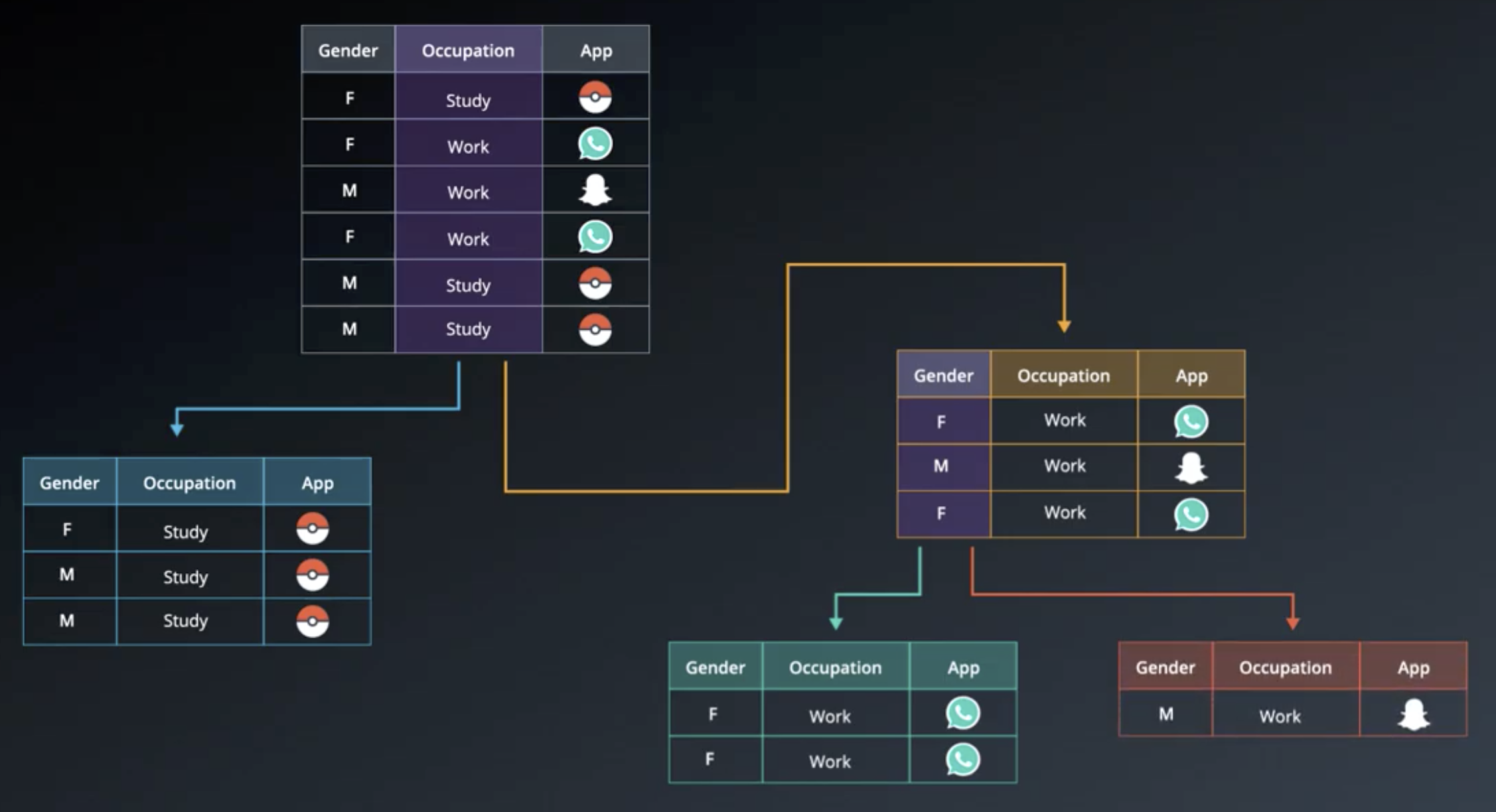
As an example, consider a table of characteristics about people and their favorite app.

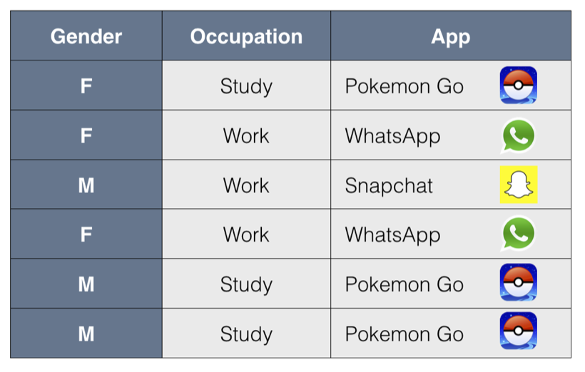
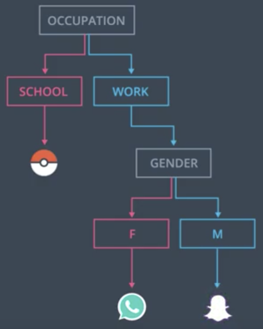
Between Gender and Occupation, the characteristic of the people that is “more decisive” for predicting what app the people will prefer is Occupation. Specifically, all students preferred the Pokemon Go app, as opposed to SnapChat and WhatsApp, the other options. Among people who work, the Gender classification can help us to determine which of the two apps they will prefer. This structure is captured in the following decision tree.

The next question: how do we get the computer to “learn” this decision tree structure from the data itself?

Student Admissions Example

Suppose that students are accepted or denied to a university based upon a combination of grade and test data. Suppose that we have the following distribution of applicants to a university.

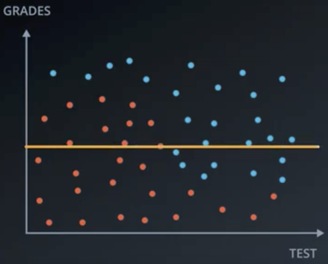
Would a horizontal line (Grade) or vertical line (Test) better split the data?

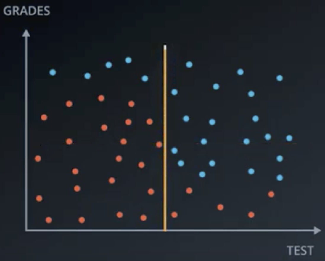
From inspection, the vertical line would better split the data, so the decision tree should begin with a filter on Test.

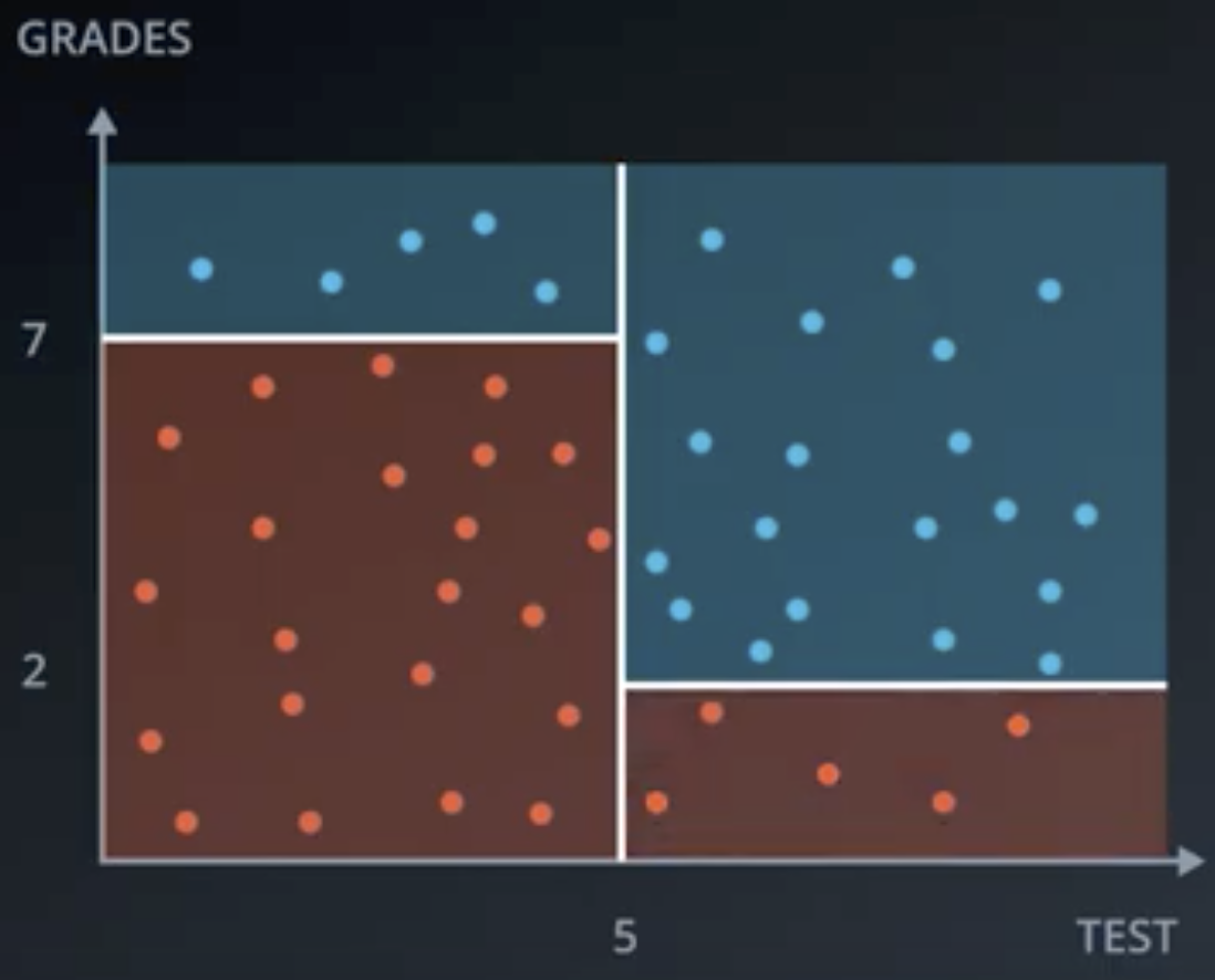
But, we can do better. By beginning with a filter on Test >= 5 then applying the criterion Grade >= 7 or Grade >= 2, depending upon the first criterion, we can split the data perfectly. Graphically, the space is split like the following.

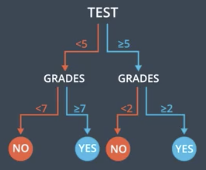
And, the decision tree looks like the following.

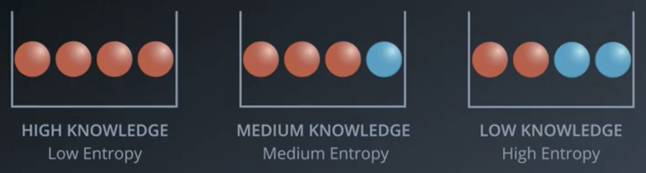
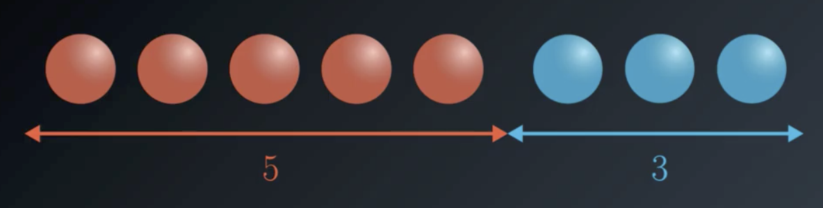
Entropy

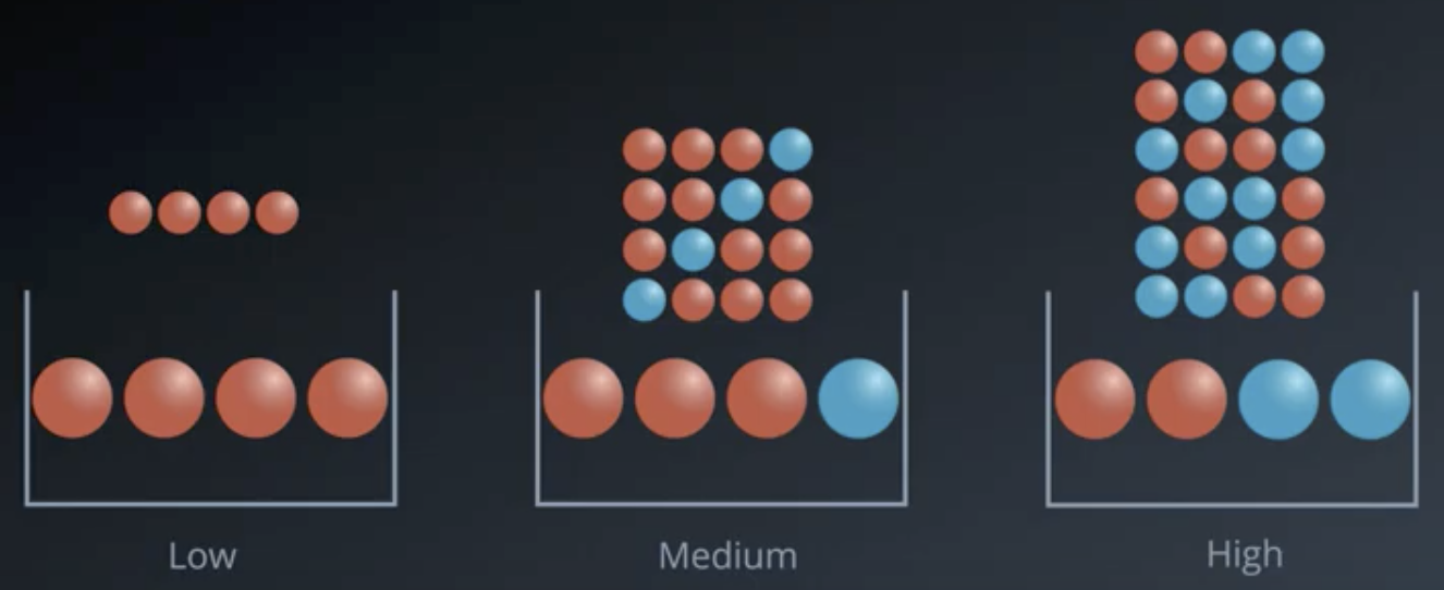
Entropy, in the context of probability, relates to the number of possible configurations that a given set of labeled data can take. Specifically, the more homogeneous a set is, the less entropy the set has. The set of four red balls can only be arranged one way, so it has relatively low entropy. The set of two red and two blue balls can be arranged six different ways, so it has relatively high entropy.

Entropy versus Prior Knowledge

Entropy is the exact opposite of prior knowledge based on the set composition. For example, in a situation where all four alls are red, we have perfect knowledge about which classification a single ball would be. In the case where the balls are evenly split between red and blue, we have relatively imperfect knowledge about which color a randomly selected ball would be.

Example from Set Probabilities

Consider a situation where we are given a set of four balls, three of which are red, and one of which is blue. What is the probability that four randomly-drawn balls (with replacement) will match the original configuration of the balls?

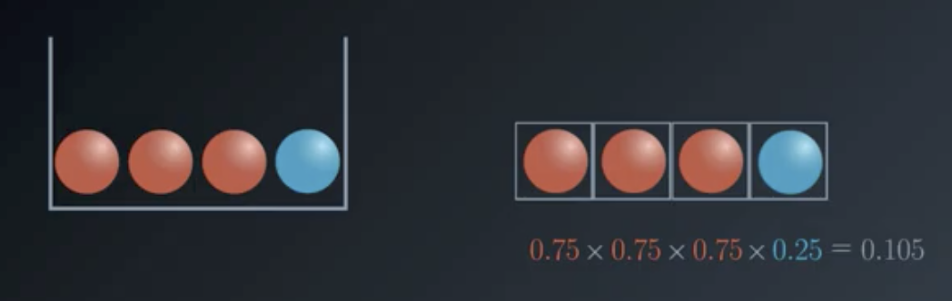
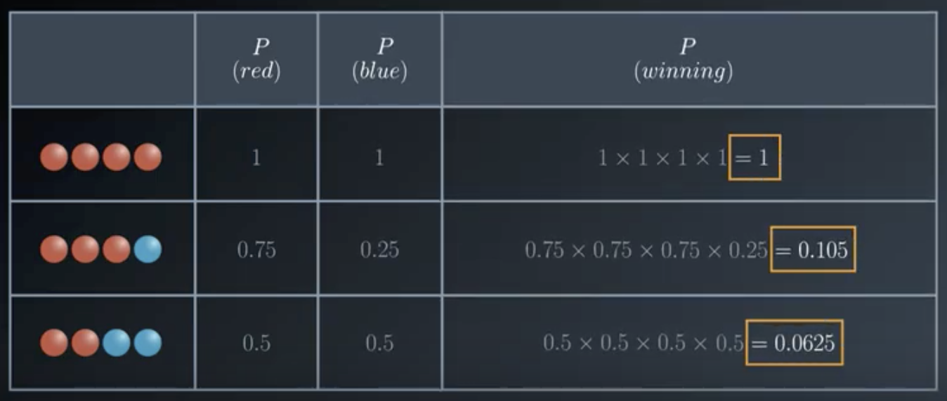
We calculate $P(R)=0.75$ and $P(B)=0.25$, so then

$$P(R,R,R,B)=0.75 \times 0.75 \times 0.75 \times 0.25 = 0.105$$

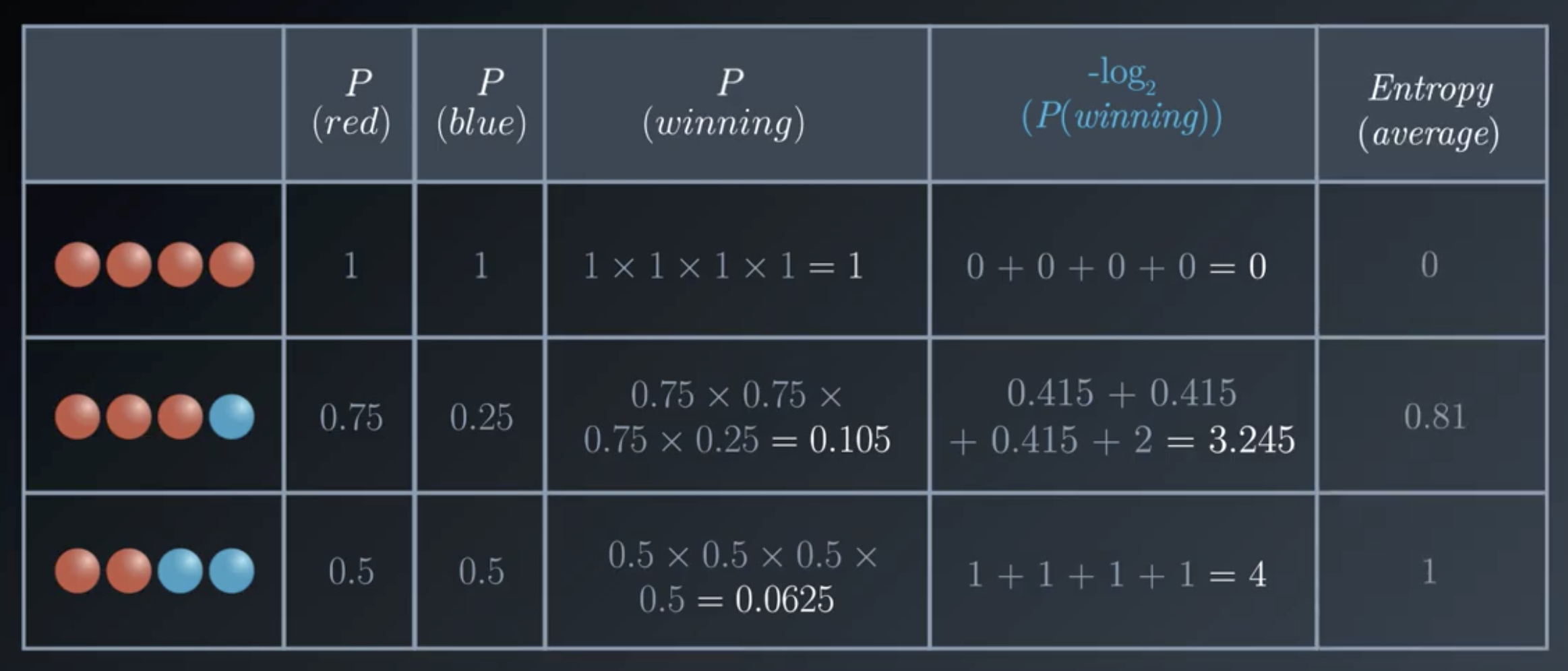
Similarly, we can fill in the rest of this table for the other configurations.

These probabilities are converted to entropy values by calculating $-log_2 (P(winning))$ and then dividing by the size of the set, resulting in the table below.

As a further example, consider a set of 8 total balls, 5 of which are red and 3 of which are blue.

Then, the entropy is given by

$$Entropy = - \frac{5}{8} log_2 (\frac{5}{8}) - \frac{3}{8} log_2 (\frac{3}{8}) = 0.9544$$

Finally, for the even more general case of $m$ red balls and $n$ blue balls

$$Entropy = - \frac{m}{m+n} log_2 (\frac{m}{m+n}) - \frac{n}{m+n} log_2 (\frac{n}{m+n})$$

For an example of 4 red balls and 10 blue balls:

$$Entropy = - \frac{4}{4+10} log_2 (\frac{4}{4+10}) - \frac{10}{4+10} log_2 (\frac{10}{4+10}) = 0.863$$

Entropy in Terms of Probabilities

The formula for entropy, above, can be rewritten in terms of the probabilities of each occurrence, as follows. Let $p_1$ stand for the probability of drawing a red ball, and $p_2$ stand for the probability of drawing a blue ball.

$$p_1 = \frac{m}{m+n};\ \ \ p_2 = \frac{n}{m+n}$$

The entropy formula can then be rewritten as

$$entropy = -p_1 log_2 (p_1) - p_2 log_2 (p_2)$$

This formula can be extended to the multi-class case, where there are three or more possible values:

$$entropy = - p_1 log_2 (p_1) - p_2 log_2 (p_2) - … - p_n log_2 (p_n) = \sum_{i=1}^n p_i log_2 (p_i)$$

Note the minimum is still 0 when all elements are the same value. The maximum is still achieved when the outcome probabilities are the same, but the upper limit increases with the number of different outcomes.

For example, consider an example with 8 red balls, 3 blue balls, and 2 yellow balls.

$$p_r = \frac{8}{13} = 0.615;\ \ \ p_b = \frac{3}{13} = 0.231;\ \ \ p_y = \frac{2}{13} = 0.154$$

$$entropy = - p_r log_2 (p_r) - p_b log_2 (p_b) - p_y log_2 (p_y) = 1.335$$

Information Gain

Information Gain is defined as a change in entropy.

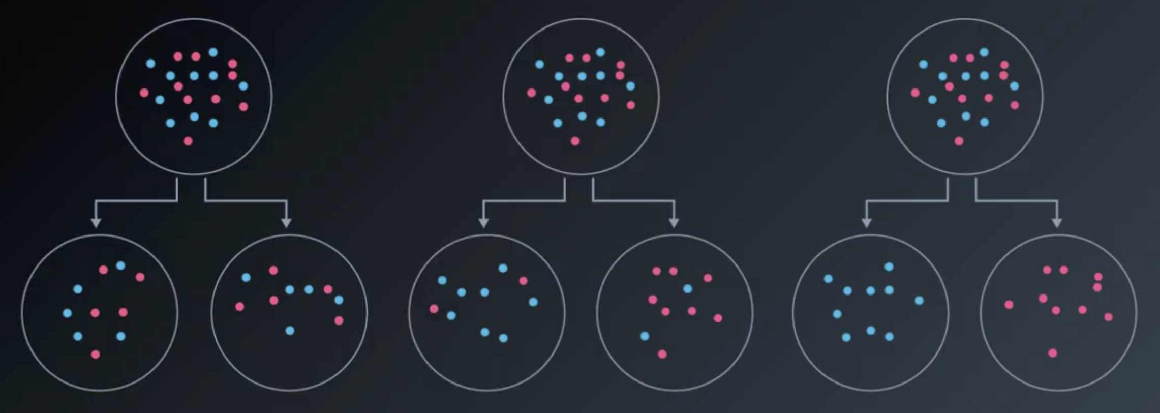
From left to right, there is a small information gain, a medium information gain, and a large information gain.

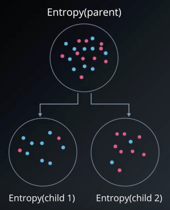
More specifically, the information gain of a given split on the data is the difference between the entropy of the parent set and the weighted average entropy of the children sets, following the split. For $m$ items in the first child group and $n$ items in the second child group, the information gain is:

$$Information\ Gain = Entropy(Parent) - [\frac{m}{m+n} Entropy(Child_1) + \frac{n}{m+n} Entropy(Child_2)]$$

Applying Information Gain to the App Preferences Example

The entropy of the starting set, above, is 1.46.

Following a split on gender, the average weighted entropy of the child sets is 0.92. So, the information gain is $1.46-0.92=0.54$.

Following a split on occupation, the average weighted entropy of the child sets is 0.46. So, the information gain is $1.46-0.46=1.00$. This provides quantitative backup for the intuition we had earlier: splitting on occupation is the best first split.

A decision tree that perfectly classifies the app preferences is shown below.

Decision Tree Hyperparameters

Maximum Depth

The max_depth of a decision tree is the largest length between the root and the leaf.

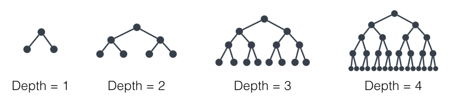
A large depth can cause overfitting, since a tree that is too deep can memorize the data. On the other hand, a small depth can result in very simple model which may be overfit.

Minimum Number of Samples to Split

A node must have at least min_samples_split in order to be large enough to split. If a node has fewer, the splitting process stops. Note that min_samples_split does not control the minimum size of leaves.

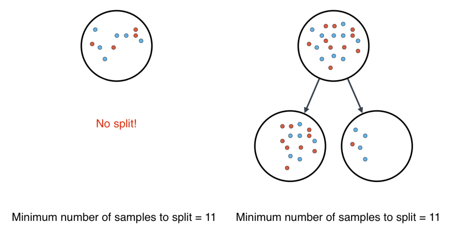
A small minimum samples per split may result in a complicated, highly branched tree which may mean the tree has memorized the data. A large minimum samples parameter may result in the tree not having enough flexibility to get built, which may result in underfitting.

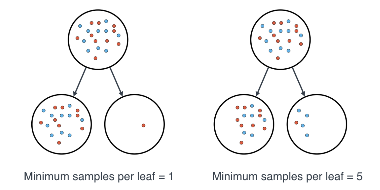
Minimum Number of Samples per Leaf

Tbe min_samples_leaf hyperparameter exists to ensure that the decision tree does not end up with 99 samples in one leaf and 1 in the other. If a threshold on a feature results in a leaf that has fewer than min_samples_leaf, the algorithm will not allow the split. But, it may perform a split on the same feature at a different threshold that does satisfy min_samples_leaf.

min_samples_per_leaf accepts both integers and floats. If an integer is provided, the parameter is taken as the number of samples per leaf. If a float is provided, the parameter is taken as the smallest fraction of overall samples in the dataset (for example, 0.10 = 10%).