Neural Network Implementations
This page shows implementations of the basic functions of the Gradient Descent algorithms and uses them to find the boundary in a small dataset.
import matplotlib.pyplot as plt
import numpy as np
import pandas as pd
Basic Functions
Sigmoid Activation Function
$$\sigma(x) = \frac{1}{1+e^{-x}}$$
def sigmoid(x):

    return 1 / (1 + np.exp(-1 * x))
Output (prediction) formula
$$\hat{y} = \sigma(w_1 x_1 + w_2 x_2 + b)$$
def output_formula(features, weights, bias):

    return sigmoid(np.dot(features, weights) + bias)
Error function
$$Error(y, \hat{y}) = - y \log(\hat{y}) - (1-y) \log(1-\hat{y})$$
def error_formula(y, output):

    return -1 * y * np.log(output) - (1 - y) * np.log(1-output)
The function that updates the weights
$$ w_i \longrightarrow w_i + \alpha (y - \hat{y}) x_i$$
$$ b \longrightarrow b + \alpha (y - \hat{y})$$
def update_weights(x, y, weights, bias, learnrate):
    output = output_formula(x, weights, bias)
    error = - (y - output)
    updated_weights = weights - learnrate * error * x
    updated_bias = bias - learnrate * error

    return updated_weights, updated_bias
Helper Functions
def plot_points(X, y):
    admitted = X[np.argwhere(y==1)]
    rejected = X[np.argwhere(y==0)]

    plt.scatter([s[0][0] for s in rejected],
                [s[0][1] for s in rejected],
                s = 25,
                color = 'blue',
                edgecolor = 'k')
    plt.scatter([s[0][0] for s in admitted],
                [s[0][1] for s in admitted],
                s = 25,
                color = 'red',
                edgecolor = 'k')
def display(m, b, color='g--'):
    plt.xlim(-0.05,1.05)
    plt.ylim(-0.05,1.05)
    x = np.arange(-10, 10, 0.1)
    plt.plot(x, m*x+b, color, alpha = 0.35)
Training Function
def train(features, targets, epochs, learnrate, graph_lines=False):
plt.figure(figsize=[11,8.5])
errors = []
n_records, n_features = features.shape
last_loss = None
weights = np.random.normal(scale=1 / n_features**.5, size=n_features)
bias = 0
for e in range(epochs):
del_w = np.zeros(weights.shape)
for x, y in zip(features, targets):
output = output_formula(x, weights, bias)
error = error_formula(y, output)
weights, bias = update_weights(x, y, weights, bias, learnrate)
# Printing out the log-loss error on the training set
out = output_formula(features, weights, bias)
loss = np.mean(error_formula(targets, out))
errors.append(loss)
if e % (epochs / 10) == 0:
print("\n========== Epoch", e,"==========")
if last_loss and last_loss < loss:
print("Train loss: ", loss, " WARNING - Loss Increasing")
else:
print("Train loss: ", loss)
last_loss = loss
predictions = out > 0.5
accuracy = np.mean(predictions == targets)
print("Accuracy: ", accuracy)
if graph_lines and e % (epochs / 100) == 0:
display(-weights[0]/weights[1], -bias/weights[1])
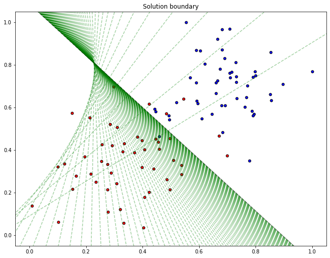
# Plotting the solution boundary
plt.title("Solution boundary")
display(-weights[0]/weights[1], -bias/weights[1], 'black')
# Plotting the data
plot_points(features, targets)
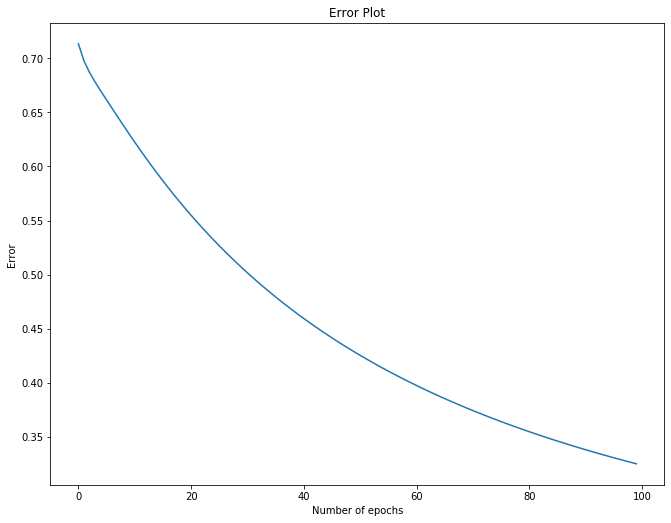
# Plotting the error
plt.figure(figsize=[11,8.5])
plt.title("Error Plot")
plt.xlabel('Number of epochs')
plt.ylabel('Error')
plt.plot(errors)
plt.show()
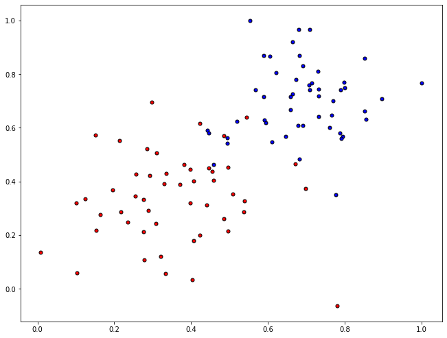
Read the Data
data = pd.read_csv('neural-network-implementations/data/data.csv', header=None)
X = np.array(data[[0,1]])
y = np.array(data[2])
plt.figure(figsize=[11,8.5])
plot_points(X,y)
Train the “Model”
np.random.seed(44)

epochs = 100
learnrate = 0.01

train(X, y, epochs, learnrate, True)
========== Epoch 0 ==========
Train loss:  0.7135845195381634
Accuracy:  0.4

========== Epoch 10 ==========
Train loss:  0.6225835210454962
Accuracy:  0.59

========== Epoch 20 ==========
Train loss:  0.5548744083669508
Accuracy:  0.74

========== Epoch 30 ==========
Train loss:  0.501606141872473
Accuracy:  0.84

========== Epoch 40 ==========
Train loss:  0.4593334641861401
Accuracy:  0.86

========== Epoch 50 ==========
Train loss:  0.42525543433469976
Accuracy:  0.93

========== Epoch 60 ==========
Train loss:  0.3973461571671399
Accuracy:  0.93

========== Epoch 70 ==========
Train loss:  0.3741469765239074
Accuracy:  0.93

========== Epoch 80 ==========
Train loss:  0.35459973368161973
Accuracy:  0.94

========== Epoch 90 ==========
Train loss:  0.3379273658879921
Accuracy:  0.94
This content is taken from notes I took while pursuing the Intro to Machine Learning with Pytorch nanodegree certification.