Neural Network Admissions Example
In this example, I predict student admissions to graduate school at UCLA based on three pieces of data:
- GRE Scores (Test)
- GPA Scores (Grades)
- Class Rank (1-4)
The dataset was originally taken from this link: http://www.ats.ucla.edu/ but may have been modified by Udacity.
Load Data
%matplotlib inline
import pandas as pd
import numpy as np
import matplotlib.pyplot as plt
d = pd.read_csv('neural-network-admissions-example/data/student_data.csv')
print(str(d.shape[0]) + ' rows')
d.head()
400 rows
| admit | gre | gpa | rank | |
|---|---|---|---|---|
| 0 | 0 | 380 | 3.61 | 3 |
| 1 | 1 | 660 | 3.67 | 3 |
| 2 | 1 | 800 | 4.00 | 1 |
| 3 | 1 | 640 | 3.19 | 4 |
| 4 | 0 | 520 | 2.93 | 4 |
Plot the Data
First, ignore the rank, so the plot is 2-dimensional.
def plot_points(d):
    plt.figure(figsize=[6,4.75])

    X = np.array(d[["gre","gpa"]])
    y = np.array(d["admit"])

    admitted = X[np.argwhere(y==1)]
    rejected = X[np.argwhere(y==0)]

    plt.scatter([s[0][0] for s in rejected],
                [s[0][1] for s in rejected],
                s = 50,
                color = 'red',
                label = 'Denied',
                alpha=0.35)

    plt.scatter([s[0][0] for s in admitted],
                [s[0][1] for s in admitted],
                s = 50,
                color = 'darkblue',
                label = 'Admitted',
                alpha=0.35)

    plt.legend(
    fancybox=True,
    loc=3,
    facecolor='white',
    edgecolor='white')

    plt.xlabel('Test (GRE)')
    plt.ylabel('Grades (GPA)')
plot_points(d)
plt.title('All Ranks');
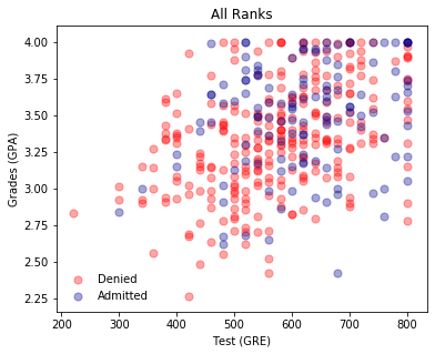
Roughly, it looks like students with higher grades and test scores were admitted. But, the data is clearly not linearly separable. The rank may help us to make more sense of the data.
First, separate the ranks into different subsets of the data. Then, plot using each subset.
d1 = d[d["rank"]==1]
d2 = d[d["rank"]==2]
d3 = d[d["rank"]==3]
d4 = d[d["rank"]==4]

plot_points(d1)
plt.title("Rank 1")
plt.show()
plot_points(d2)
plt.title("Rank 2")
plt.show()
plot_points(d3)
plt.title("Rank 3")
plt.show()
plot_points(d4)
plt.title("Rank 4")
plt.show()
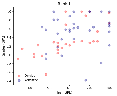
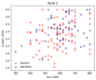
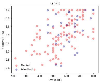
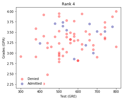
It appears that the lower the rank, the higher the acceptances. It makes sense to use the rank as one of the inputs. To do this, we will need to one-hot encode it.
One-hot Encoding the Rank
Use Panda’s get_dummies.
one_hot_data = pd.get_dummies(d,
                              columns=['rank'])
one_hot_data.head()
| admit | gre | gpa | rank_1 | rank_2 | rank_3 | rank_4 | |
|---|---|---|---|---|---|---|---|
| 0 | 0 | 380 | 3.61 | 0 | 0 | 1 | 0 |
| 1 | 1 | 660 | 3.67 | 0 | 0 | 1 | 0 |
| 2 | 1 | 800 | 4.00 | 1 | 0 | 0 | 0 |
| 3 | 1 | 640 | 3.19 | 0 | 0 | 0 | 1 |
| 4 | 0 | 520 | 2.93 | 0 | 0 | 0 | 1 |
Scale the Data
Fit both the GRE and GPA data into a range of 0-1 by dividing the grades by 4.0 and the test score by 800.
processed_data = one_hot_data
processed_data['gre'] /= 800
processed_data['gpa'] /= 4.
processed_data.head()
| admit | gre | gpa | rank_1 | rank_2 | rank_3 | rank_4 | |
|---|---|---|---|---|---|---|---|
| 0 | 0 | 0.475 | 0.9025 | 0 | 0 | 1 | 0 |
| 1 | 1 | 0.825 | 0.9175 | 0 | 0 | 1 | 0 |
| 2 | 1 | 1.000 | 1.0000 | 1 | 0 | 0 | 0 |
| 3 | 1 | 0.800 | 0.7975 | 0 | 0 | 0 | 1 |
| 4 | 0 | 0.650 | 0.7325 | 0 | 0 | 0 | 1 |
Split the Data into Training and Testing
The example below does not use Sklearn’s train_test_split to demonstrate an alternative method.
sample = np.random.choice(processed_data.index,
                          size=int(len(processed_data)*0.9),
                          replace=False)
train_data, test_data = processed_data.iloc[sample], processed_data.drop(sample)
print('Training Data: {} rows'.format(train_data.shape[0]))
print(' Testing Data:  {} rows'.format(test_data.shape[0]))
Training Data: 360 rows
 Testing Data:  40 rows
Split the data into Features and Labels
features = train_data.drop(columns=['admit'])
targets = train_data['admit']
features_test = test_data.drop(columns=['admit'])
targets_test = test_data['admit']
Training the 2-Layer Neural Network
First, some utility functions.
Sigmoid Activation Function
def sigmoid(x):

    return 1 / (1 + np.exp(-x))
Derivative of Sigmoid Activation Function
def sigmoid_prime(x):

    return sigmoid(x) * (1-sigmoid(x))
Error Function
def error_formula(y, output):

    return - y*np.log(output) - (1 - y) * np.log(1-output)
Error Term Formula
$$Error\ Term = -(y-\hat{y})\sigma `(x)$$
def error_term_formula(y, output):

    return (y-output) * output * (1 - output)
Backpropagate the Error
# Neural Network hyperparameters
epochs = 1000
learnrate = 0.5

# Training function
def train_nn(features, targets, epochs, learnrate):

    # Use to same seed to make debugging easier
    np.random.seed(42)

    n_records, n_features = features.shape
    last_loss = None

    # Initialize weights
    weights = np.random.normal(scale=1 / n_features**.5, size=n_features)

    for e in range(epochs):
        del_w = np.zeros(weights.shape)
        for x, y in zip(features.values, targets):
            # Loop through all records, x is the input, y is the target

            # Activation of the output unit
            #   Notice we multiply the inputs and the weights here
            #   rather than storing h as a separate variable
            output = sigmoid(np.dot(x, weights))

            # The error, the target minus the network output
            error = error_formula(y, output)

            # The error term
            #   Calulate f'(h) here instead of defining a separate
            #   sigmoid_prime function. This just makes it faster because we
            #   can re-use the result of the sigmoid function stored in
            #   the output variable
            error_term = error_term_formula(y, output)

            del_w += error_term * x

        # Update the weights here. The learning rate times the
        # change in weights, divided by the number of records to average
        weights += learnrate * del_w / n_records

        # Printing out the mean square error on the training set
        if e % (epochs / 10) == 0:
            out = sigmoid(np.dot(features, weights))
            loss = np.mean((out - targets) ** 2)
            print("Epoch:", e)
            if last_loss and last_loss < loss:
                print("Train loss: ", loss, "  WARNING - Loss Increasing")
            else:
                print("Train loss: ", loss)
            last_loss = loss
            print("=========")
    print("Finished training!")
    return weights

weights = train_nn(features, targets, epochs, learnrate)
Epoch: 0
Train loss:  0.27322921091147634
=========
Epoch: 100
Train loss:  0.2047581256002055
=========
Epoch: 200
Train loss:  0.20255452027395668
=========
Epoch: 300
Train loss:  0.20153969072910288
=========
Epoch: 400
Train loss:  0.2010100178416723
=========
Epoch: 500
Train loss:  0.20068356425817008
=========
Epoch: 600
Train loss:  0.20044728889319113
=========
Epoch: 700
Train loss:  0.20025427734771004
=========
Epoch: 800
Train loss:  0.20008402998279995
=========
Epoch: 900
Train loss:  0.199927063762658
=========
Finished training!
Calculate the Accuracy on the Test Data
tes_out = sigmoid(np.dot(features_test, weights))
predictions = tes_out > 0.5
accuracy = np.mean(predictions == targets_test)
print("Prediction accuracy: {:.3f}".format(accuracy))
Prediction accuracy: 0.625