Multilayer Perceptrons

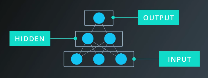
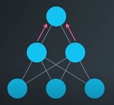
Adding a “hidden” layer of perceptrons allows the model to find solutions to linearly inseparable problems. An example of this architecture is shown below.

The input to the hidden layer is the same as it was before, as is the the activation function.

$$h_j = \sum_i w_{ij} \times x_i + b_j$$

$$a_j = sigmoid(h_j)$$

The input to the output layer is the output of the hidden layer.

$$o_k = \sum_j w_{jk} \times a_j + b_j$$

$$a_k = sigmoid(o_k)$$

Stacking more and more layers helps the network learn more patterns. This is where the term “deep learning” comes from.

Neural Network Mathematics

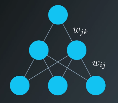
The following notation will be used for the weights: $w_{ij}$ where $i$ denotes input units and $j$ denotes the hidden units.

For example, the following image shows are network with input units labeled $x_1$, $x_2$, and $x_3$, and hidden nodes labeled $h_1$ and $h_2$.

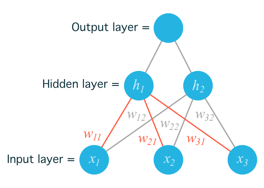
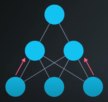
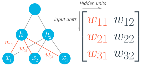
The weights need to be stored in a matrix, indexed as $w_{ij}$. Each row in the matrix corresponds to the weights leading out of a single input unit, and each column corresponds to the weights leading into a single hidden unit.

To initialize these weights we need the shape of the matrix. If we have a 2D array called features containing the input data:

n_records, n_inputs = features.shape
n_hidden = 2
weights_input_to_hidden = np.random.normal(0, n_inputs**-0.5, size=(n_inputs, n_hidden))

The result is a 2D array (or, “matrix”) named weights_input_to_hidden with dimensions n_inputs by n_hidden. Recall that the input to a hidden unit is the sum of all the inputs multiplied by the hidden unit’s weights. So, for each hidden unit, $h_j$, we use linear algebra to calculate the following sum.

$$h_j=\sum_i w_{ij} x_i$$

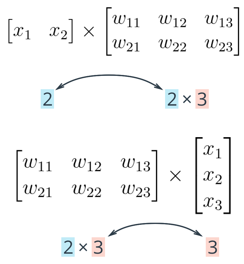
For the architecture described above, we’re multiplying the input (a row vector) by the weights (a matrix). This is accomplished by taking the dot product of the inputs with each column in the weights matrix. The following is for the input to the first hidden unit, $j=1$, which is associated to the first column of the weights matrix.

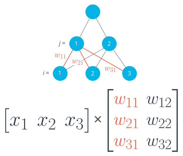
$$h_1=x_1 w_{11} + x_2 w_{21} + x_3 w_{31}$$

The sum of products for the second hidden layer output would be similar, except using the dot product of the inputs with the second column, and so on. Using Numpy, this calculation can be run for all the inputs and outputs simultaneously:

hidden_inputs = np.dot(inputs, weights_input_to_hidden)

Note that the weights matrix could also be defined as follows, with dimensions n_hidden by n_inputs, then multiply by a inputs when set up as a column vector. Note that the weight indices no longer match up with the labels used in earlier diagrams. In matrix notation, the row index always precedes the column index.

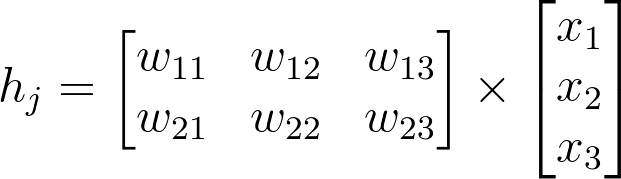
The critical thing to remember with matrix multiplication is that the dimensions must match. For example, three columns in the input vector, and three rows in the weights matrix. Here’s the rule:

• If multiplying an array from the left, the array must have the same number of elements as there are rows in the matrix.
• If multiplying the matrix from the left, the number of columns in the matrix must equal the number of elements in the array on the right.