Gradient Descent Implementations

10 May 2020

Single Update Example

From the gradient descent notes, we saw that one weight update is calculated as:

$$\Delta w_i = \eta \delta x_i$$

The error term $\delta$ is given by:

$$\delta = (y - \hat{y}) f'(h) = (y-\hat{y}) f'(\sum w_i x_i)$$

In the error term, $(y-\hat{y})$ is the output error, $f'(h)$ refers to the derivative of the activation function, which is $f(h)$. We will refer to $f'(h)$ as the output gradient.

import numpy as np

def sigmoid(x):
    """
    Calculate sigmoid
    """
    return 1/(1+np.exp(-x))

def sigmoid_prime(x):
    """
    # Derivative of the sigmoid function
    """
    return sigmoid(x) * (1 - sigmoid(x))

learnrate = 0.5
x = np.array([1, 2, 3, 4])
y = np.array(0.5)

# Initial weights
w = np.array([0.5, -0.5, 0.3, 0.1])

Calculate one gradient descent step for each weight

# Calculate the node's linear combination of inputs and weights
h = np.dot(x, w)

# Calculate output of neural network
nn_output = sigmoid(h)

# Calculate error of neural network
error = y - nn_output

# Calculate the error term
error_term = error * sigmoid_prime(h)

# Calculate change in weights
del_w = learnrate * error_term * x

print('Neural Network output: {:1.3f}'.format(nn_output))
print('      Amount of Error: {:1.3f}'.format(error))
print('    Change in Weights: ' + str(del_w))

Neural Network output: 0.690
      Amount of Error: -0.190
    Change in Weights: [-0.02031869 -0.04063738 -0.06095608 -0.08127477]

Graduate School Admissions Example

From this point, this page is very similar to the Neural Network Admissions Example. It relies on the same base data and contains much of the same code.

The code in the previous section demonstrated how to update weights for a single update:

$$\Delta w_{ij} = \eta \delta_j x_i$$

The next section will demonstrate how to perform many updates to fully optimize a neural network.

Data Cleanup and Splitting

The data must be cleaned up and transformed before it can be used. This cleanup consists of two steps:

Standardize GRE and GPA, which makes them have a zero mean and a standard deviation of 1.
Encode the Rank categorical variable [(1, 2, 3, 4)] using one-hot encoding [(1, 0, 0, 0), (0, 1, 0, 0), …].

import pandas as pd

admissions = pd.read_csv('gradient-descent-implementations/data/data.csv')

print('raw admissions: ' + str(admissions.shape[0]) + ' rows')
admissions.head()

raw admissions: 400 rows

	admit	gre	gpa	rank
0	0	380	3.61	3
1	1	660	3.67	3
2	1	800	4.00	1
3	1	640	3.19	4
4	0	520	2.93	4

# Make dummy variables for rank
data = pd.concat([admissions, pd.get_dummies(admissions['rank'], prefix='rank')], 
                 axis=1)
data = data.drop(columns=['rank'])

# Standarize features
for field in ['gre', 'gpa']:
    mean, std = data[field].mean(), data[field].std()
    data.loc[:,field] = (data[field]-mean)/std

print('data: ' + str(data.shape[0]) + ' rows')
data.head()

data: 400 rows

	admit	gre	gpa	rank_1	rank_3	rank_4
0	0	-1.798011	0.578348	0	1	0
1	1	0.625884	0.736008	0	1	0
2	1	1.837832	1.603135	1	0	0
3	1	0.452749	-0.525269	0	0	1
4	0	-0.586063	-1.208461	0	0	1

# Split off random 10% of the data for testing
np.random.seed(42)
sample = np.random.choice(data.index, size=int(len(data)*0.9), replace=False)
data, test_data = data.iloc[sample], data.drop(sample)

# Split into features and targets
features, targets = data.drop(columns=['admit']), data['admit']
features_test, targets_test = test_data.drop(columns=['admit']), test_data['admit']

print('     features: ' + str(features.shape[0]) + ' rows')
print('features_test: ' + str(features_test.shape[0]) + ' rows')
features.head()

     features: 360 rows
features_test: 40 rows

	gre	gpa	rank_2	rank_3	rank_4
209	-0.066657	0.289305	1	0	0
280	0.625884	1.445476	1	0	0
33	1.837832	1.603135	0	1	0
210	1.318426	-0.131120	0	0	1
93	-0.066657	-1.208461	1	0	0

Mean Squared Error

Instead of using the Sum of Squared Errors (SSE), we will be using the Mean Squared Error (MSE). When using larger datasets, summing up all the weight steps can lead to very large updates that make the gradient descent diverge. To compensate for this, it would be necessary to use a very small learning rate.

Instead of using this small learning rate, we can just divide by the number of records in the data, $m$, to take the average. This ensures that no matter how much data is used, the learning rates will usually be between 0.01 and 0.001. Then, we can use the MSE to calculate the gradient and the result will be the same as before.

$$E = \frac{1}{2m} sum_\mu (y^\mu - \hat{y}^\mu)^2$$

General algorithm for updating the weights with gradient descent

Set the weight step to zero: $\Delta w_i = 0$
For each record in the training data:
- Make a forward pass through the network, calculating the output: $\hat{y}=f(\sum_i w_i x_i)$
- Calculate the error term for the output unit: $\delta = (y-\hat{y}) f'(\sum_i w_i x_i)$
- Update the weight step $\Delta w_i = \Delta w_i + \delta x_i$
Update the weights $w_i = w_i + \eta \Delta w_i / m$ where: $\eta$ is the learning rate, $m$ is the number of records. Average the weight steps to reduce any large variations in the training data.
Repeat for $e$ epochs.

An alternative approach would be to update the weights on each record instead of average the weight steps after going through all the records.

Recall that we are using sigmoid as the activation function, $f(h) = \frac{1}{1+e^{-h}}$.

The gradient of the sigmoid is $f'(h)=f(h)(1-f(h))$.

$h$ is the input to the output unit: $h=\sum_i w_i x_i$

Implemention Notes

The first step in the implementation is to initialize the weights. These need to be:

small, so they are in the linear region near zero and not at the high and low ends,
random, so they have different starting values and diverge.

A normal distribution centered at 0 with scale $\frac{1}{\sqrt(n)}$, where $n$ is the number of input units, meets these criteria.

n_records, n_features = features.shape
print('n_records, n_features: {}, {}'.format(n_records, n_features))
weights = np.random.normal(scale=1/n_features**.5, size=n_features)

n_records, n_features: 360, 6

The input to the output layer will be calculated using Numpy’s dot() function, which performs multiplication on two arrays element-wise (1st element $\times$ 1st element, etc) and then sums those products.

# input to the output layer
output_in = np.dot(weights, features.iloc[0])

Implementing Gradient Descent

Setup

weights_df, delta_weights_df = (pd.DataFrame(columns=features.columns), 
                                pd.DataFrame(columns=features.columns))

def sigmoid(x):
    """
    Calculate sigmoid
    """
    return 1 / (1 + np.exp(-x))

# Use to same seed to make debugging easier
np.random.seed(42)

n_records, n_features = features.shape
last_loss = None

# Initialize weights
weights = np.random.normal(scale=1 / n_features**.5, size=n_features)

# Neural Network hyperparameters
epochs = 5001
learnrate = 0.1

Gradient Descent

for e in range(epochs):
    
    del_w = np.zeros(weights.shape)
    
    for x, y in zip(features.values, targets):
        # Loop through all records, x is the input, y is the target

        output = sigmoid(np.dot(weights, x))

        error = y-output

        error_term = error * output * (1 - output)

        del_w += error_term * x

    weights += learnrate * del_w / n_records

    # Printing out the mean square error on the training set
    if e % (int(epochs / 10)) == 0:
        out = sigmoid(np.dot(features, weights))
        loss = np.mean((out - targets) ** 2)
        if last_loss and last_loss < loss:
            print("Epoch {:4} - Train loss: {:1.5f} WARNING - Loss Increasing"
                  .format(e,loss))
        else:
            print("Epoch {:4} - Train loss: {:1.5f}".format(e,loss))
        last_loss = loss
    
    # Save weights and weight change for plotting later
    weights_df = (weights_df
                  .append(
                      pd.DataFrame(weights.reshape(1,-1),
                                   columns=features.columns)))
    delta_weights_df = (delta_weights_df
                        .append(
                            pd.DataFrame(del_w.reshape(1,-1),
                                         columns=features.columns)))

Epoch    0 - Train loss: 0.26390
Epoch  500 - Train loss: 0.20948
Epoch 1000 - Train loss: 0.20090
Epoch 1500 - Train loss: 0.19864
Epoch 2000 - Train loss: 0.19781
Epoch 2500 - Train loss: 0.19743
Epoch 3000 - Train loss: 0.19724
Epoch 3500 - Train loss: 0.19713
Epoch 4000 - Train loss: 0.19707
Epoch 4500 - Train loss: 0.19703
Epoch 5000 - Train loss: 0.19701

Calculate accuracy on test data

tes_out = sigmoid(np.dot(features_test, weights))
predictions = tes_out > 0.5
accuracy = np.mean(predictions == targets_test)
print("\nPrediction accuracy: {:2.1%}".format(accuracy))

Prediction accuracy: 72.5%

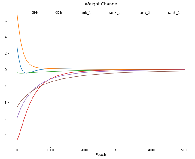
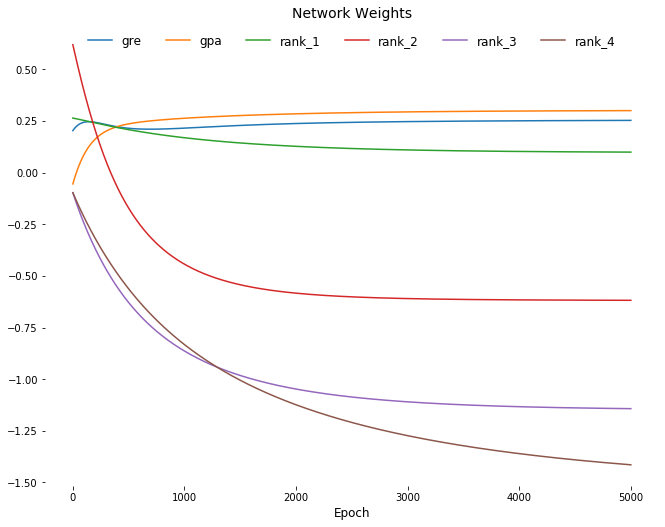
Visualize

import matplotlib.pyplot as plt

weights_df = weights_df.reset_index(drop=True)
delta_weights_df = delta_weights_df.reset_index(drop=True)

plt.figure(figsize=[11,8.5])

for col in weights_df.columns:
    plt.plot(weights_df.index,
             weights_df[[col]],
             label=col);

plt.title('Network Weights', fontsize=14)
plt.xlabel('Epoch', fontsize=12)

for spine in plt.gca().spines.values():
    spine.set_visible(False)

plt.legend(
fancybox=True,
loc=9,
ncol=6,
facecolor='white',
edgecolor='white',
framealpha=1,
fontsize=12);

png

plt.figure(figsize=[11,8.5])

for col in weights_df.columns:
    plt.plot(delta_weights_df.index,
             delta_weights_df[[col]],
             label=col);
    
plt.title('Weight Change', fontsize=14)
plt.xlabel('Epoch', fontsize=12)

for spine in plt.gca().spines.values():
    spine.set_visible(False)

plt.legend(
fancybox=True,
loc=9,
ncol=6,
facecolor='white',
edgecolor='white',
framealpha=1,
fontsize=12);

png

This content is taken from notes I took while pursuing the Intro to Machine Learning with Pytorch nanodegree certification.