financial advice. You should do your own research before making any decisions.
Bitcoin 4-Year SMA Analysis
According to Michael Saylor, “The best #bitcoin price signal for technocrats or maximalists is the 4 year simple moving average.” A live 4-Year SMA chart courtesy of Buy Bitcoin Worldwide is linked here.
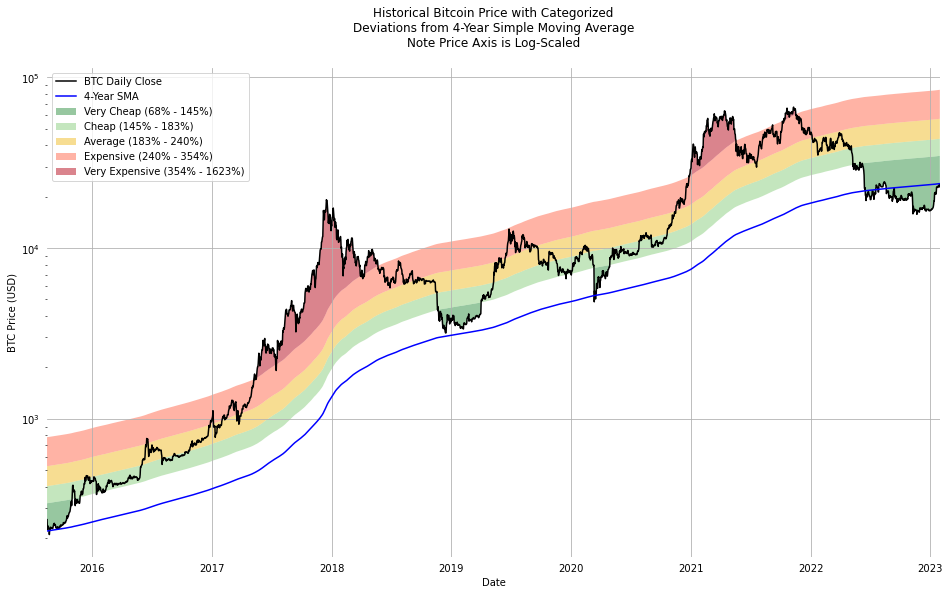
The objective of the analysis on this page is to derive a straightforward categorization scheme for historical bitcoin price deviations relative to the 4-year simple moving average price.
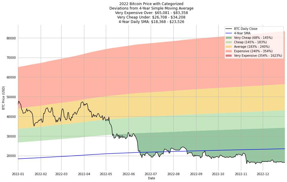
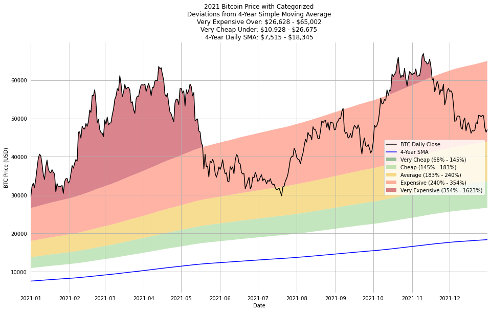
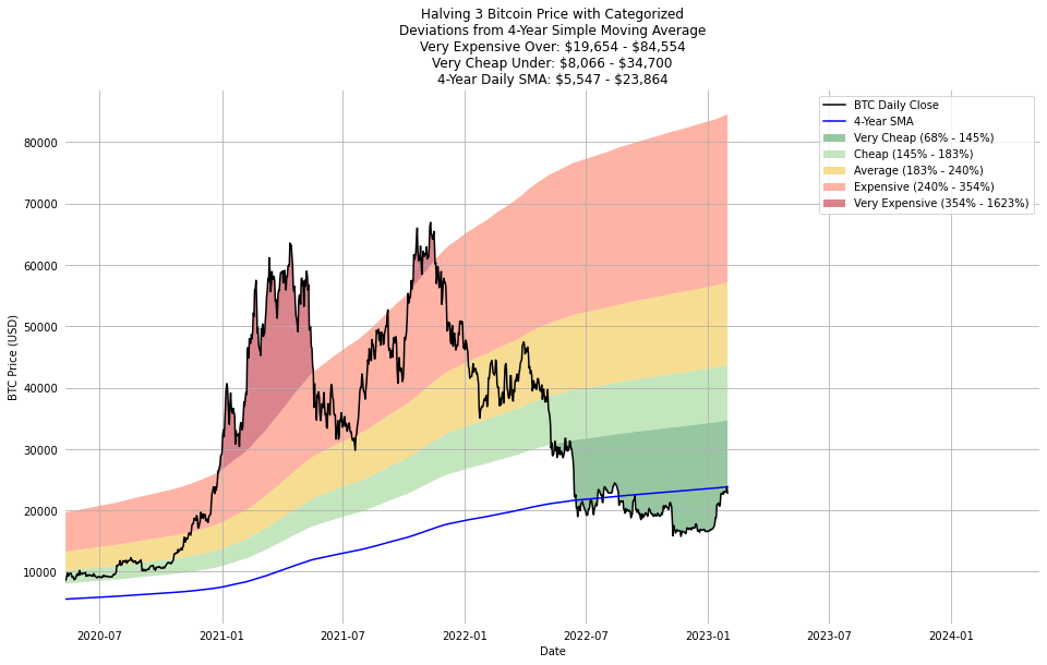
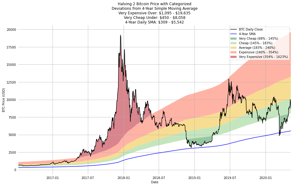
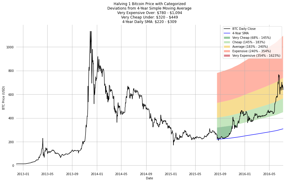
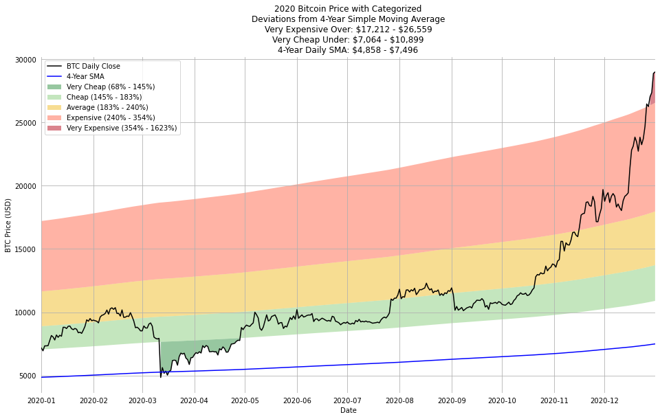
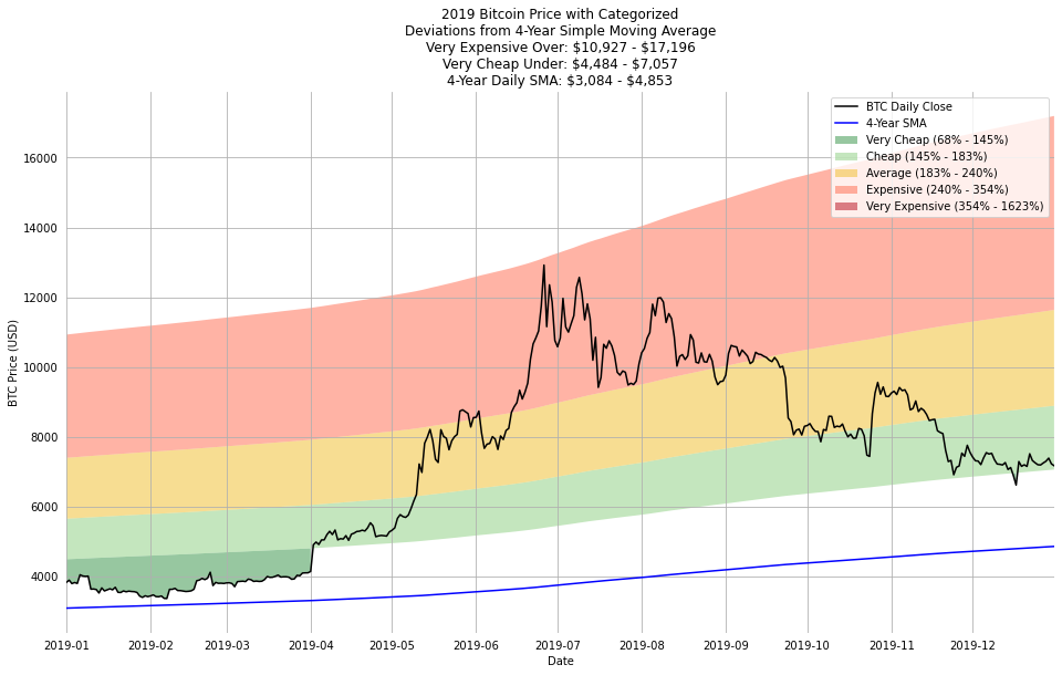
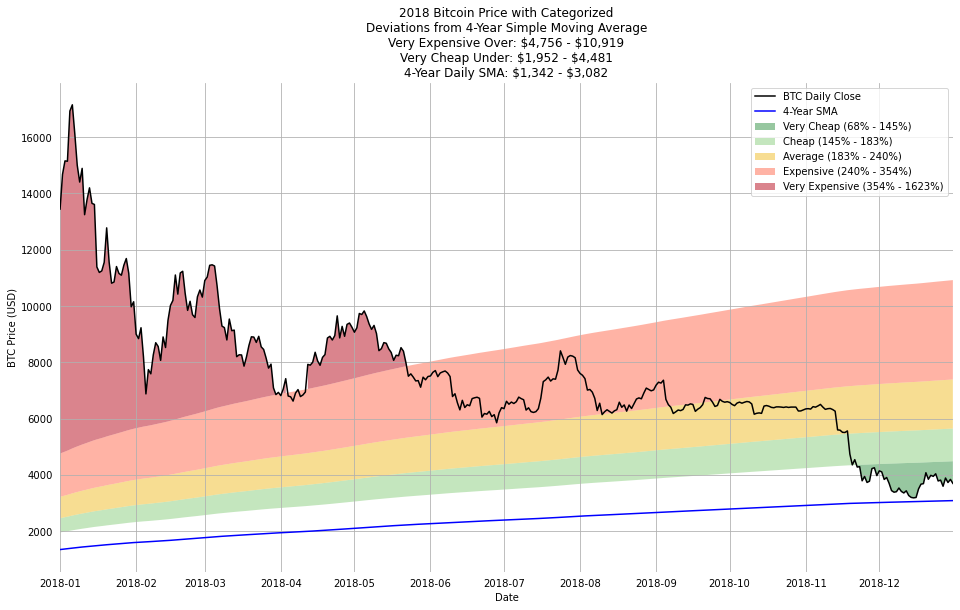
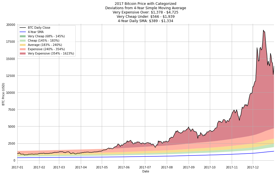
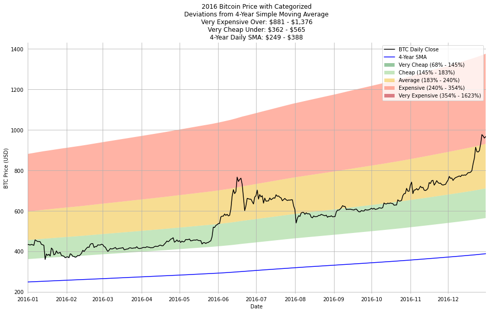
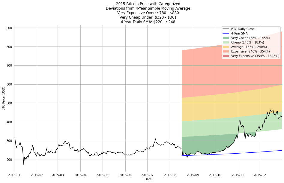
The outcome of this analysis is a set of annual, by-halving, and total price history visuals of this 5-tier price classification scheme since August 2015, which is when a 4-year SMA for the bitcoin price was first calculable. The thresholds for the classifications are updated daily, so over the course of each timeframe the thresholds are a range.
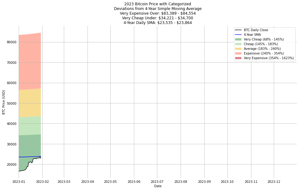
As of 2023-01-30, the thresholds for this classification scheme are:
- Very Cheap: Under \$34,700
- Cheap: Under \$43,700
- Average: Under \$57,200
- Expensive: Under \$84,600
- Very Expensive: Over \$84,600
Results of this Analysis
The price classifications and daily closing price are presented below for all available price history, 2023, 2022, 2021, halvings 1 and 2, and all available price history, and at the bottom of this page for 2015-2023, halvings 1-3, and all available price history.
Possible Acquisition Strategies
The following is not financial advice - do your own research and make your own decisions.
Fixed Allocation
If the long term goal is to acquire and hold an increasing amount of bitcoin while also preserving a USD cash buffer, its reasonable to consider a strategy of maintaining a fixed ratio of cash relative to the dollar value of BTC owned. Practically, following this strategy would mean using free cash flow to buy Bitcoin as required to maintain the desired ratio. This is a very practical way to “buy the dip” without becoming too emotionally involved. For example, a person targeting a 10% fixed allocation would keep \$5000 cash on hand per BTC owned when it is trading at \$50K, but would decrease their cash position (effectively spending the delta buying the dip) to \$3000 per BTC if it traded down to \$30K.
Dynamic Allocation
One way to potentially improve upon the “fixed % allocation” strategy just outlined would be to increase the BTC allocation when BTC is relatively “cheap,” and decrease the BTC allocation when it becomes relatively “expensive.” As an example, someone with target cash-to-bitcoin ratios of 10% to 20% could consider keeping a 10% cash buffer when BTC is “very cheap” according to the classification scheme outlined on this page, and 20% when BTC trades up and gets “very expensive.” This way, when BTC drops they opportunitistically buy the dip, and when BTC trades up they stash cash (ie, “dry powder”.)
Practically, as a point-in-time example, a person using the ratios above could consider the following target cash positions:
- If BTC price is Very Cheap, keep cash = 10% of less than \$34.7K = less than \$3,500 per 1 BTC
- If BTC price is Cheap, keep cash = 12.5% of \$34.7K to \$43.7K = \$4,300 to \$5,500 per 1 BTC
- If BTC price is Average, keep cash = 15% of \$43.7K to \$57.2K = \$6,600 to \$8,600 per 1 BTC
- If BTC price is Expensive, keep cash = 17.5% of \$57.2K to \$84.6K = \$10,000 to \$14,800 per 1 BTC
- If BTC price is Very Expensive, keep cash = 20% of \$84.6K = more than \$16,900 per 1 BTC
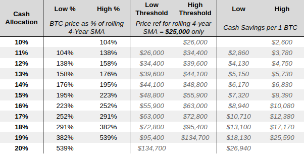
The following table shows a 5-tier target cash allocation scheme with BTC price thresholds based on a \$25K 4-year SMA.

A second table below shows a similar 11-tier scheme with BTC price thresholds based on a $25K 4-year SMA.
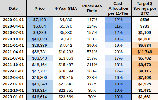
The table below has target cash allocations for the past few years based on the 11-tier scheme. The historical pricing and SMA values are taken from this chart.
Continously Variable Allocation
Obviously the % allocation toward dollars could instead be calculated to vary continuously as a function of the deviation from the 4-year SMA. And obviously one’s BTC balance (denominated in BTC) would increase over time. The thresholds for relative cheapness would also change due to BTC price action. This whole structure is very multivariate.
The examples in the preceding section are just snapshot, point-in-time worked examples intended to outline a possible framework for mitigating risks of BTC price action without being too emotionally involved.
Other Charts from the 5-Tier Classification Scheme
Open Raw Data
Data from August 18, 2011 until August 2, 2021 was taken from a tradingview.com export of Bitcoin pricing from the Bitstamp exchange. Data after August 2, 2021 was taken from an API pull of pricing data from CoinAPI.
import datetime as dt
from datetime import date
import pandas as pd
import matplotlib.pyplot as plt
import numpy as np
import matplotlib as mpl
d = pd.read_csv('bitcoin-4-year-sma-analysis/btc_daily_closing_price.csv')
print('Earliest date: {}\nLatest date: {}\n'.format(d['time'].min()[:10],
                                                    d['time'].max()[:10]))
d.info()
d.head()
Earliest date: 2011-08-18
Latest date: 2023-01-30

<class 'pandas.core.frame.DataFrame'>
RangeIndex: 4151 entries, 0 to 4150
Data columns (total 2 columns):
 #   Column  Non-Null Count  Dtype
---  ------  --------------  -----
 0   time    4151 non-null   object
 1   close   4151 non-null   float64
dtypes: float64(1), object(1)
memory usage: 65.0+ KB
| time | close | |
|---|---|---|
| 0 | 2011-08-18 | 10.90 |
| 1 | 2011-08-19 | 11.69 |
| 2 | 2011-08-20 | 11.70 |
| 3 | 2011-08-21 | 11.70 |
| 4 | 2011-08-22 | 11.70 |
d.tail()
| time | close | |
|---|---|---|
| 4146 | 2023-01-26 | 23017.91025 |
| 4147 | 2023-01-27 | 23075.51994 |
| 4148 | 2023-01-28 | 23035.20209 |
| 4149 | 2023-01-29 | 23755.85993 |
| 4150 | 2023-01-30 | 22836.34803 |
Basic Cleansing
- Convert “time” to “date”
- Identify any missing days by merging into a complete list of dates from the start to end date
d['date'] = pd.to_datetime(d['time'])
complete_date_list = pd.DataFrame(
    pd.date_range(dt.datetime(2011, 8, 18),
                  dt.datetime(2024, 5, 12)),
    columns=['date'])
print(d.shape)
d = (pd.merge(complete_date_list, d,
              on=['date'],
              how='left')
     .reset_index(drop=True))
print(d.shape)
(4151, 3)
(4652, 3)
d = (d[['date','close']]
     .reset_index(drop=True))
d.info()
<class 'pandas.core.frame.DataFrame'>
RangeIndex: 4652 entries, 0 to 4651
Data columns (total 2 columns):
 #   Column  Non-Null Count  Dtype
---  ------  --------------  -----
 0   date    4652 non-null   datetime64[ns]
 1   close   4151 non-null   float64
dtypes: datetime64[ns](1), float64(1)
memory usage: 72.8 KB
Exploration & Cleansing
- A total of 33 days are missing pricing information. This is less than 1% of the total values in the dataset, and 30/33 were in 2011. Clean by filling the values forward.
d[(d['close'].isna())&
  (d['date'] <= dt.datetime(2022, 9, 24))]['date'].dt.year.value_counts()
2011    30
2015     3
Name: date, dtype: int64
d.loc[d['date'] <= dt.datetime(2022, 9, 24), 'close'] = d['close'].fillna(method='ffill')
d.info()
<class 'pandas.core.frame.DataFrame'>
RangeIndex: 4652 entries, 0 to 4651
Data columns (total 2 columns):
 #   Column  Non-Null Count  Dtype
---  ------  --------------  -----
 0   date    4652 non-null   datetime64[ns]
 1   close   4184 non-null   float64
dtypes: datetime64[ns](1), float64(1)
memory usage: 72.8 KB
Label Halvings
d.loc[ d['date'].dt.date <  date.fromisoformat('2012-11-28'),  'halving'] = 0
d.loc[(d['date'].dt.date >= date.fromisoformat('2012-11-28'))&
      (d['date'].dt.date <  date.fromisoformat('2016-07-09')), 'halving'] = 1
d.loc[(d['date'].dt.date >= date.fromisoformat('2016-07-09'))&
      (d['date'].dt.date <  date.fromisoformat('2020-05-11')), 'halving'] = 2
d.loc[(d['date'].dt.date >= date.fromisoformat('2020-05-11')), 'halving'] = 3
d['halving'] = d['halving'].astype(int)
d = d[['date','halving','close']].reset_index(drop=True)
d.info()
<class 'pandas.core.frame.DataFrame'>
RangeIndex: 4652 entries, 0 to 4651
Data columns (total 3 columns):
 #   Column   Non-Null Count  Dtype
---  ------   --------------  -----
 0   date     4652 non-null   datetime64[ns]
 1   halving  4652 non-null   int64
 2   close    4184 non-null   float64
dtypes: datetime64[ns](1), float64(1), int64(1)
memory usage: 109.2 KB
Calculate 4-Year Simple Moving Averages
365.25 days/year * 4 years = 1461 days. Calculate % delta from the 4-year SMA as well.
d['sma_1461'] = (d['close']
                 .rolling(window=1461)
                 .mean())
d['% delta'] = (d['close'] / d['sma_1461']) * 100.
d.info()
<class 'pandas.core.frame.DataFrame'>
RangeIndex: 4652 entries, 0 to 4651
Data columns (total 5 columns):
 #   Column    Non-Null Count  Dtype
---  ------    --------------  -----
 0   date      4652 non-null   datetime64[ns]
 1   halving   4652 non-null   int64
 2   close     4184 non-null   float64
 3   sma_1461  2724 non-null   float64
 4   % delta   2724 non-null   float64
dtypes: datetime64[ns](1), float64(3), int64(1)
memory usage: 181.8 KB
Split into five equally-populated categories.
d['category'] = pd.qcut(d['% delta'],
                        5,
                        labels=['Very Cheap','Cheap',
                                'Average',
                                'Expensive','Very Expensive'])
d['cuts'] = pd.qcut(d['% delta'],
                    5)
limits = (d[['close','category','cuts']]
          .groupby(['category','cuts'])
          .count()
          .replace(0,np.nan)
          .dropna()
          .reset_index()
          .rename(columns={'close':'# days'}))
limits['low'] = (limits['cuts'].astype(str)
                 .str.replace('(','',
                              regex=False)
                 .str.split(', ',
                            expand=True)[0])
limits['high'] = (limits['cuts'].astype(str)
                  .str.replace(']','',
                               regex=False)
                  .str.split(', ',
                             expand=True)[1])
limits['category label'] = ((limits['category'].astype(str) + ' (' +
                             (limits['low'].astype(float)
                              .round(0).astype(int).astype(str)) + '% - ' +
                             (limits['high'].astype(float)
                              .round(0).astype(int).astype(str)) + '%)'))
limits
| category | cuts | # days | low | high | category label | |
|---|---|---|---|---|---|---|
| 0 | Very Cheap | (68.03399999999999, 145.406] | 545.0 | 68.03399999999999 | 145.406 | Very Cheap (68% - 145%) |
| 1 | Cheap | (145.406, 183.112] | 545.0 | 145.406 | 183.112 | Cheap (145% - 183%) |
| 2 | Average | (183.112, 239.734] | 544.0 | 183.112 | 239.734 | Average (183% - 240%) |
| 3 | Expensive | (239.734, 354.319] | 545.0 | 239.734 | 354.319 | Expensive (240% - 354%) |
| 4 | Very Expensive | (354.319, 1622.743] | 545.0 | 354.319 | 1622.743 | Very Expensive (354% - 1623%) |
for num, low in enumerate(limits['low'].values):
    d[num+1] = d['sma_1461'] * float(low) / 100.
pd.DataFrame(d[(d['date'] == dt.datetime(2023, 1, 30))].T)
| 4183 | |
|---|---|
| date | 2023-01-30 00:00:00 |
| halving | 3 |
| close | 22836.34803 |
| sma_1461 | 23863.87848 |
| % delta | 95.694202 |
| category | Very Cheap |
| cuts | (68.03399999999999, 145.406] |
| 1 | 16235.551085 |
| 2 | 34699.511143 |
| 3 | 43697.625163 |
| 4 | 57209.830436 |
| 5 | 84554.255593 |
def print_plot(sub, timeframe, time_increment):
    plt.figure(figsize=(16,9), facecolor='white')

    mpl.rcParams['axes.prop_cycle'] = mpl.cycler(color=['#309143', '#8ace7e',
                                                        '#f0bd27',
                                                        '#ff684c', '#b60a1c'])
    plt.plot(pd.to_datetime(sub['date']),
             sub['close'],
             color='k',
             label='BTC Daily Close',
             linewidth=1.5)
    plt.plot(pd.to_datetime(sub['date']),
             sub['sma_1461'],
             color='blue',
             alpha=1,
             label='4-Year SMA',
             linewidth=1.5)
    plt.xlim(sub.iloc[0]['date'], sub.iloc[-1]['date'])

    plt.fill_between(sub['date'],
                     sub[2],
                     sub['close'],
                     where=sub['close'] < sub[2],
                     label=limits['category label'].values[0],
                     alpha=0.5)
    for col in d.columns[9:]:
        plt.fill_between(sub['date'],
                         sub[col],
                         sub[col-1],
                         label=limits['category label'].values[col-2],
                         alpha=0.5)
    plt.fill_between(sub['date'],
                     sub[5],
                     sub['close'],
                     where=sub['close'] > sub[5],
                     label=limits['category label'].values[4],
                     alpha=0.5)

    plt.gca().tick_params(top=False,
                          bottom=False,
                          left=False,
                          right=False,
                          labelleft=True,
                          labelbottom=True)
    for spine in plt.gca().spines.values():
        spine.set_visible(False)
    plt.grid()

    title = '''Deviations from 4-Year Simple Moving Average
Very Expensive Over: \${:,.0f} - ${:,.0f}
Very Cheap Under: \${:,.0f} - ${:,.0f}
4-Year Daily SMA: \${:,.0f} - ${:,.0f}'''.format(round(sub[5].min(),3),
                                                 round(sub[5].max(),3),
                                                 round(sub[2].min(),3),
                                                 round(sub[2].max(),3),
                                                 round(sub['sma_1461'].min(),3),
                                                 round(sub['sma_1461'].max(),3))

    if time_increment == 'year':
        title = '''{} Bitcoin Price with Categorized
'''.format(timeframe) + title
    elif time_increment == 'halving':
        title = '''Halving {} Bitcoin Price with Categorized
'''.format(timeframe) + title
    else:
        plt.yscale("log")
        title = '''Historical Bitcoin Price with Categorized
Deviations from 4-Year Simple Moving Average
Note Price Axis is Log-Scaled
'''

    plt.title(title)
    plt.legend()
    plt.ylabel('BTC Price (USD)')
    plt.xlabel('Date');
for year in ['2023','2022','2021','2020',
             '2019','2018','2017','2016',
             '2015']:
    sub = d[d['date'].astype(str).str.contains(year)].copy()
    print_plot(sub, year, 'year')
for halving in [3, 2, 1]:
    sub = d[d['halving']==halving].copy()
    print_plot(sub, halving, 'halving')
print_plot(d[~d['sma_1461'].isna()], '', 'total_history')