Ridge, Lasso, and Polynomial Linear Regression
Ridge Regression
Ridge regression learns $w$, $b$ using the same least-squares criterion but adds a penalty for large variations in $w$ parameters.
$$RSS_{RIDGE}(w,b)=\sum_{(i=1)}^N (y_i-(w \cdot x_i + b))^2 + \alpha \sum_{(j=1)}^p w_j^2$$
The addition of a penalty parameter is called regularization. Regularization is an important concept in machine learning. It is a way to prevent overfitting by reducing the model complexity. It improves the likely generalization performance of a model by restricting the model’s possible parameter settings.
The practical effect of using ridge regression is to find feature weights, $w$, that fit the data well and also set many of the feature weights to small values. The accuracy improvement on a regression problem with dozens or hundreds of features is significant.
The influence of the regularization term is controlled by the $\alpha$ parameter, where larger $\alpha$ means more regularization and simpler models. The default $\alpha$ value is 1.
from sklearn.model_selection import train_test_split
from sklearn.linear_model import Ridge

X_train, X_test, y_train, y_test = train_test_split(X_crime, y_crime,
                                                   random_state = 0)

linridge = Ridge(alpha=20.0).fit(X_train, y_train)

print('Crime dataset')
print('ridge regression linear model intercept: {}'
     .format(linridge.intercept_))
print('ridge regression linear model coeff:\n{}'
     .format(linridge.coef_))
print('R-squared score (training): {:.3f}'
     .format(linridge.score(X_train, y_train)))
print('R-squared score (test): {:.3f}'
     .format(linridge.score(X_test, y_test)))
print('Number of non-zero features: {}'
     .format(np.sum(linridge.coef_ != 0)))
Crime dataset
ridge regression linear model intercept: -3352.4230358463437
ridge regression linear model coeff:
[ 1.95091438e-03  2.19322667e+01  9.56286607e+00 -3.59178973e+01
  6.36465325e+00 -1.96885471e+01 -2.80715856e-03  1.66254486e+00
 -6.61426604e-03 -6.95450680e+00  1.71944731e+01 -5.62819154e+00
  8.83525114e+00  6.79085746e-01 -7.33614221e+00  6.70389803e-03
  9.78505502e-04  5.01202169e-03 -4.89870524e+00 -1.79270062e+01
  9.17572382e+00 -1.24454193e+00  1.21845360e+00  1.03233089e+01
 -3.78037278e+00 -3.73428973e+00  4.74595305e+00  8.42696855e+00
  3.09250005e+01  1.18644167e+01 -2.05183675e+00 -3.82210450e+01
  1.85081589e+01  1.52510829e+00 -2.20086608e+01  2.46283912e+00
  3.29328703e-01  4.02228467e+00 -1.12903533e+01 -4.69567413e-03
  4.27046505e+01 -1.22507167e-03  1.40795790e+00  9.35041855e-01
 -3.00464253e+00  1.12390514e+00 -1.82487653e+01 -1.54653407e+01
  2.41917002e+01 -1.32497562e+01 -4.20113118e-01 -3.59710660e+01
  1.29786751e+01 -2.80765995e+01  4.38513476e+01  3.86590044e+01
 -6.46024046e+01 -1.63714023e+01  2.90397330e+01  4.15472907e+00
  5.34033563e+01  1.98773191e-02 -5.47413979e-01  1.23883518e+01
  1.03526583e+01 -1.57238894e+00  3.15887097e+00  8.77757987e+00
 -2.94724962e+01 -2.33454302e-04  3.13528914e-04 -4.13169509e-04
 -1.80309962e-04 -5.74054525e-01 -5.17742507e-01 -4.20670933e-01
  1.53383596e-01  1.32725423e+00  3.84863158e+00  3.03024594e+00
 -3.77692644e+01  1.37933464e-01  3.07676522e-01  1.57128807e+01
  3.31418306e-01  3.35994414e+00  1.61265911e-01 -2.67619878e+00]
R-squared score (training): 0.671
R-squared score (test): 0.494
Number of non-zero features: 88
Feature Preprocessing and Normalization
The effect of increasing $\alpha$ is to shrink the $w$ coefficients towards 0 and toward each other. But, if the features have very different scales, then they will also have very different contributions to the penalty. So, transforming the input features so they are all on the same scale means the the ridge penalty is applied more “fairly” to all all features without unduly weighting some more than others just do to a difference in scales.
The Need for Feature Normalization
It is important for some machine learning methods that all features are on the same scale. This can result in faster convergence in learning and assigning more uniform or “fair” influence for all weights. This is true specifically for regularized regression, k-NN, support vector machines, and neural networks.
The need for feature normalization can also depend on the data, which is a broader subject called feature engineering.
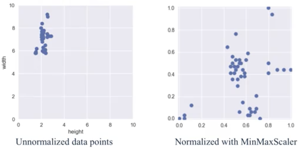
One widely-used type of feature scaling is called MinMax scaling. It transforms the features so they are all on the same scale between 0 and 1:
- For each feature $x_i$: compute the minimum value $x_i^{MIN}$ and maximum value $x_i^{MAX}$ in the dataset.
- For each feature $x_i$: transform a given feature $x_i$ value to a scaled version $x_i^{\prime}$ using the following formula:
$$x_i^{\prime}=\frac{x_i-x_i^{MIN}}{x_i^{MAX}-x_i^{MIN}}$$
from sklearn.preprocessing import MinMaxScaler
scaler = MinMaxScaler()

from sklearn.linear_model import Ridge
X_train, X_test, y_train, y_test = train_test_split(X_crime, y_crime,
                                                    random_state = 0)

X_train_scaled = scaler.fit_transform(X_train)
X_test_scaled = scaler.transform(X_test)
Note:
- The same scalar object is applied to both the training and test sets, and
- We are training the scalar object on the training data and not on the test data.
These are crucial aspects to feature normalization.
- Fit the scalar using the training set, then apply the same scalar to transform the test set.
- Do not scale the training and test sets using different scalars. This could lead to random skew in the data.
- Do not fit the scalar using any part of the test data. Referencing the test data can lead to a form of data leakage, where the training phase has inofrmation that is leaked from the test set.
MinMax scaling is not the only type of feature normalization that’s best to apply. The choice of feature normalization that’s best to apply depends on the data set, learning task, and learning algorithm to be used.
linridge = Ridge(alpha=20.0).fit(X_train_scaled, y_train)

print('Crime dataset')
print('ridge regression linear model intercept: {}'
     .format(linridge.intercept_))
print('ridge regression linear model coeff:\n{}'
     .format(linridge.coef_))
print('R-squared score (training): {:.3f}'
     .format(linridge.score(X_train_scaled, y_train)))
print('R-squared score (test): {:.3f}'
     .format(linridge.score(X_test_scaled, y_test)))
print('Number of non-zero features: {}'
     .format(np.sum(linridge.coef_ != 0)))
Crime dataset
ridge regression linear model intercept: 933.3906385044156
ridge regression linear model coeff:
[  88.68827454   16.48947987  -50.30285445  -82.90507574  -65.89507244
   -2.27674244   87.74108514  150.94862182   18.8802613   -31.05554992
  -43.13536109 -189.44266328   -4.52658099  107.97866804  -76.53358414
    2.86032762   34.95230077   90.13523036   52.46428263  -62.10898424
  115.01780357    2.66942023    6.94331369   -5.66646499 -101.55269144
  -36.9087526    -8.7053343    29.11999068  171.25963057   99.36919476
   75.06611841  123.63522539   95.24316483 -330.61044265 -442.30179004
 -284.49744001 -258.37150609   17.66431072 -101.70717151  110.64762887
  523.13611718   24.8208959     4.86533322  -30.46775619   -3.51753937
   50.57947231   10.84840601   18.27680946   44.11189865   58.33588176
   67.08698975  -57.93524659  116.1446052    53.81163718   49.01607711
   -7.62262031   55.14288543  -52.08878272  123.39291017   77.12562171
   45.49795317  184.91229771  -91.35721203    1.07975971  234.09267451
   10.3887921    94.7171829   167.91856631  -25.14025088   -1.18242839
   14.60362467   36.77122659   53.19878339  -78.86365997   -5.89858411
   26.04790298  115.1534917    68.74143311   68.28588166   16.5260514
  -97.90513652  205.20448474   75.97304123   61.3791085   -79.83157049
   67.26700741   95.67094538  -11.88380569]
R-squared score (training): 0.615
R-squared score (test): 0.599
Number of non-zero features: 88
Note that following MinMax scaling, the R-squared score increased from 0.494 to 0.599.
In general, regularization works well , when the amount of data is relatively small compared to the number of features in the model. Regularization becomes less important as the amount of training data increases.
The following example of varying alpha demonstrates the general relationship between model complexity and test set performance.
for this_alpha in [0, 1, 10, 20, 50, 100, 1000]:
    linridge = Ridge(alpha = this_alpha).fit(X_train_scaled, y_train)
    r2_train = linridge.score(X_train_scaled, y_train)
    r2_test = linridge.score(X_test_scaled, y_test)
    num_coeff_bigger = np.sum(abs(linridge.coef_) > 1.0)
    print('Alpha = {:.0f}:\tnum abs(coeff) > 1.0: {},\tr-squared training, test: {:.0f}, {:.2f}\r'
         .format(this_alpha, num_coeff_bigger, r2_train, r2_test))
Alpha = 0:	num abs(coeff) > 1.0: 88,	r-squared training, test: 1, 0.50
Alpha = 1:	num abs(coeff) > 1.0: 87,	r-squared training, test: 1, 0.56
Alpha = 10:	num abs(coeff) > 1.0: 87,	r-squared training, test: 1, 0.59
Alpha = 20:	num abs(coeff) > 1.0: 88,	r-squared training, test: 1, 0.60
Alpha = 50:	num abs(coeff) > 1.0: 86,	r-squared training, test: 1, 0.58
Alpha = 100:	num abs(coeff) > 1.0: 87,	r-squared training, test: 1, 0.55
Alpha = 1000:	num abs(coeff) > 1.0: 84,	r-squared training, test: 0, 0.30
Lasso Regression
Lasso regression is another form of regularized linear regression that uses an L1 regularization penalty for training, instead of the L2 regularization penalty used by Ridge regression.
$$RSS_{LASSO}(w,b)=\sum_{(i=1)}^N (y_i-(w \cdot x_i + b))^2 + \alpha \sum_{(j=1)}^p |w_j|$$
This has the effect of setting parameter weights in $w$ to zero for the least influential variables, called a “sparse solution.”
When to use ridge versus lasso regression:
- Use Ridge if there are only a few variables with many small/medium sized effects.
- Use Lasso if there are only a few variables with medium/large effects.
from sklearn.linear_model import Lasso
scaler = MinMaxScaler()

X_train, X_test, y_train, y_test = train_test_split(X_crime, y_crime,
                                                    random_state = 0)

X_train_scaled = scaler.fit_transform(X_train)
X_test_scaled = scaler.transform(X_test)

linlasso = Lasso(alpha=2.0, max_iter = 10000).fit(X_train_scaled, y_train)

print('Crime dataset')
print('lasso regression linear model intercept: {}'
     .format(linlasso.intercept_))
print('lasso regression linear model coeff:\n{}'
     .format(linlasso.coef_))
print('Non-zero features: {}'
     .format(np.sum(linlasso.coef_ != 0)))
print('R-squared score (training): {:.3f}'
     .format(linlasso.score(X_train_scaled, y_train)))
print('R-squared score (test): {:.3f}\n'
     .format(linlasso.score(X_test_scaled, y_test)))
print('Top Features with non-zero weight:')

for e in sorted (list(zip(list(X_crime), linlasso.coef_)),
                key = lambda e: -abs(e[1])):
    if e[1] != 0:
        print('\t{}, {:.3f}'.format(e[0], e[1]))
Crime dataset
lasso regression linear model intercept: 1186.612061998579
lasso regression linear model coeff:
[    0.             0.            -0.          -168.18346054
    -0.            -0.             0.           119.6938194
     0.            -0.             0.          -169.67564456
    -0.             0.            -0.             0.
     0.             0.            -0.            -0.
     0.            -0.             0.             0.
   -57.52991966    -0.            -0.             0.
   259.32889226    -0.             0.             0.
     0.            -0.         -1188.7396867     -0.
    -0.            -0.          -231.42347299     0.
  1488.36512229     0.            -0.            -0.
    -0.             0.             0.             0.
     0.             0.            -0.             0.
    20.14419415     0.             0.             0.
     0.             0.           339.04468804     0.
     0.           459.53799903    -0.             0.
   122.69221826    -0.            91.41202242     0.
    -0.             0.             0.            73.14365856
     0.            -0.             0.             0.
    86.35600042     0.             0.             0.
  -104.57143405   264.93206555     0.            23.4488645
   -49.39355188     0.             5.19775369     0.        ]
Non-zero features: 20
R-squared score (training): 0.631
R-squared score (test): 0.624

Top Features with non-zero weight:
	PctKidsBornNeverMar, 1488.365
	PctKids2Par, -1188.740
	HousVacant, 459.538
	PctPersDenseHous, 339.045
	NumInShelters, 264.932
	MalePctDivorce, 259.329
	PctWorkMom, -231.423
	pctWInvInc, -169.676
	agePct12t29, -168.183
	PctVacantBoarded, 122.692
	pctUrban, 119.694
	MedOwnCostPctIncNoMtg, -104.571
	MedYrHousBuilt, 91.412
	RentQrange, 86.356
	OwnOccHiQuart, 73.144
	PctEmplManu, -57.530
	PctBornSameState, -49.394
	PctForeignBorn, 23.449
	PctLargHouseFam, 20.144
	PctSameCity85, 5.198
So, 20 out of 88 features have non-zero weight in this example. The top five features with strongest relationships between input variables and outcomes for this dataset are:
- PctKidsBornNeverMar, the percentage of kids born to people who never married,
- PctKids2Par, the percentage of kids in family housing with two parents,
- HousVacant, the number of vacant houses,
- PctPersDensHous, the percetage of persons in dense housing (1+ person/room), and
- NumInShelters, the number of people in homeless shelters.
for alpha in [0.5, 1, 2, 3, 5, 10, 20, 50]:
    linlasso = Lasso(alpha, max_iter = 10000).fit(X_train_scaled, y_train)
    r2_train = linlasso.score(X_train_scaled, y_train)
    r2_test = linlasso.score(X_test_scaled, y_test)

    print('Alpha = {:.0f}:\tFeatures kept: {}\tr-squared training, test:\t{:.2f}, {:.2f}\r'
         .format(alpha, np.sum(linlasso.coef_ != 0), r2_train, r2_test))
Alpha = 0:	Features kept: 35	r-squared training, test:	0.65, 0.58
Alpha = 1:	Features kept: 25	r-squared training, test:	0.64, 0.60
Alpha = 2:	Features kept: 20	r-squared training, test:	0.63, 0.62
Alpha = 3:	Features kept: 17	r-squared training, test:	0.62, 0.63
Alpha = 5:	Features kept: 12	r-squared training, test:	0.60, 0.61
Alpha = 10:	Features kept: 6	r-squared training, test:	0.57, 0.58
Alpha = 20:	Features kept: 2	r-squared training, test:	0.51, 0.50
Alpha = 50:	Features kept: 1	r-squared training, test:	0.31, 0.30
Same as with Lasso regression, there is an optimal range of values for $\alpha$ that will be different for different data sets and different feature preprocessing methods being used.
Polynomial features with Linear Regression
Suppose we have a set of two-dimensional data points with features $x_0$ and $x_1$:
$$\textbf{x}=(x_0,x_1)$$
We could transform each data point by adding additional features that were the three unique multiplicative combinations of $x_0$ and $x_1$, yielding the following:
$$\textbf{x}=(x_0, x_1, x_0^2, x_0 x_1, x_1^2)$$
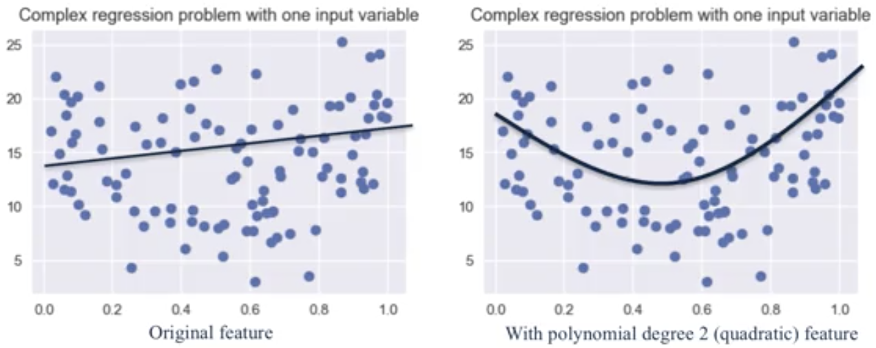
The degree of the polynomial specifies how many variables participate at a time in each new feature (above: 2). Note that this is still a weighted linear comination of features, so its still a linear model. But, this can be thought of intuitively as allowing polynomials to be fit to the training data instead of simply a straight line, but still using the same least-squares criterion.
 This approach of adding new features, such as polynomial feaures, is very effective with classification. For example, housing prices may vary as a quadratic function of both the lot size and the amount of taxes paid on the property.
It is important to be careful about polynomial feature expansion with high degree, because this can lead to complex models that overfit. For this reason, polynomial feature expansion is also combined with a regularized learning method like ridge regression.
from sklearn.linear_model import LinearRegression

X_train, X_test, y_train, y_test = train_test_split(X_F1, y_F1,
                                                    random_state = 0)
linreg = LinearRegression().fit(X_train, y_train)

print('linear model coeff (w): {}'
     .format(linreg.coef_))
print('linear model intercept (b): {:.3f}'
     .format(linreg.intercept_))
print('R-squared score (training): {:.3f}'
     .format(linreg.score(X_train, y_train)))
print('R-squared score (test): {:.3f}'
     .format(linreg.score(X_test, y_test)))
linear model coeff (w): [ 4.42036739  5.99661447  0.52894712 10.23751345  6.5507973  -2.02082636
 -0.32378811]
linear model intercept (b): 1.543
R-squared score (training): 0.722
R-squared score (test): 0.722
from sklearn.preprocessing import PolynomialFeatures

poly = PolynomialFeatures(degree=2)
X_F1_poly = poly.fit_transform(X_F1)

X_train, X_test, y_train, y_test = train_test_split(X_F1_poly, y_F1,
                                                   random_state = 0)
linreg = LinearRegression().fit(X_train, y_train)

print('(poly deg 2) linear model coeff (w):\n{}'
     .format(linreg.coef_))
print('(poly deg 2) linear model intercept (b): {:.3f}'
     .format(linreg.intercept_))
print('(poly deg 2) R-squared score (training): {:.3f}'
     .format(linreg.score(X_train, y_train)))
print('(poly deg 2) R-squared score (test): {:.3f}\n'
     .format(linreg.score(X_test, y_test)))
(poly deg 2) linear model coeff (w):
[ 3.40951018e-12  1.66452443e+01  2.67285381e+01 -2.21348316e+01
  1.24359227e+01  6.93086826e+00  1.04772675e+00  3.71352773e+00
 -1.33785505e+01 -5.73177185e+00  1.61813184e+00  3.66399592e+00
  5.04513181e+00 -1.45835979e+00  1.95156872e+00 -1.51297378e+01
  4.86762224e+00 -2.97084269e+00 -7.78370522e+00  5.14696078e+00
 -4.65479361e+00  1.84147395e+01 -2.22040650e+00  2.16572630e+00
 -1.27989481e+00  1.87946559e+00  1.52962716e-01  5.62073813e-01
 -8.91697516e-01 -2.18481128e+00  1.37595426e+00 -4.90336041e+00
 -2.23535458e+00  1.38268439e+00 -5.51908208e-01 -1.08795007e+00]
(poly deg 2) linear model intercept (b): -3.206
(poly deg 2) R-squared score (training): 0.969
(poly deg 2) R-squared score (test): 0.805
The polynomial features version appears to have overfit. Note that the R-squared score is nearly 1 on the training data, and only 0.8 on the test data. The addition of many polynomial features often leads to overfitting, so it is common to use polynomial features in combination with regression that has a regularization penalty, like ridge regression.
X_train, X_test, y_train, y_test = train_test_split(X_F1_poly, y_F1,
                                                   random_state = 0)
linreg = Ridge().fit(X_train, y_train)

print('(poly deg 2 + ridge) linear model coeff (w):\n{}'
     .format(linreg.coef_))
print('(poly deg 2 + ridge) linear model intercept (b): {:.3f}'
     .format(linreg.intercept_))
print('(poly deg 2 + ridge) R-squared score (training): {:.3f}'
     .format(linreg.score(X_train, y_train)))
print('(poly deg 2 + ridge) R-squared score (test): {:.3f}'
     .format(linreg.score(X_test, y_test)))
(poly deg 2 + ridge) linear model coeff (w):
[ 0.          2.229281    4.73349734 -3.15432089  3.8585194   1.60970912
 -0.76967054 -0.14956002 -1.75215371  1.5970487   1.37080607  2.51598244
  2.71746523  0.48531538 -1.9356048  -1.62914955  1.51474518  0.88674141
  0.26141199  2.04931775 -1.93025705  3.61850966 -0.71788143  0.63173956
 -3.16429847  1.29161448  3.545085    1.73422041  0.94347654 -0.51207219
  1.70114448 -1.97949067  1.80687548 -0.2173863   2.87585898 -0.89423157]
(poly deg 2 + ridge) linear model intercept (b): 5.418
(poly deg 2 + ridge) R-squared score (training): 0.826
(poly deg 2 + ridge) R-squared score (test): 0.825
Note that this model outperforms both the linear model and the version with polynomial features that was trained using non-regularized regression.
import pandas as pd
import numpy as np

crime_datafile = 'ridge-lasso-and-polynomial-regression/CommViolPredUnnormalizedData.txt'
crime = pd.read_table(crime_datafile,
                      sep=',',
                      na_values='?')
columns_to_keep = ([5, 6] + list(range(11,26))
                   + list(range(32, 103)) + [145])
crime = (crime[crime.columns[columns_to_keep]]
         .dropna()
         .reset_index(drop=True))
X_crime = crime[crime.columns[:88]]
y_crime = crime[crime.columns[88]]
from sklearn.datasets import make_friedman1

X_F1, y_F1 = make_friedman1(n_samples = 100,
                            n_features = 7,
                            random_state=0)